Tuesday, January 24, 2012
Idea's MRE 0, 25, 50, 75 and 100th Percentile Results
 Here are Idea's MRE results for 19 datasets since I'm missing sdr, I also added them to Ekrems MRE .CSV file results. But still working on ranking them against Ekrems results. Installed node.js and Node Packet Manager as well as coffeescript. Translated bootstrap.coffee to javascript but still haven't managed to understand it fully. Haven't been able to run bootstrap.coffee either. Looked over wilcoxonTest.awx, mwuTest.awk as well but no success.
Monday, January 23, 2012
Intrinsic Complexity of SEE
How complex should a learner working on SEE data sets be? Our intuition is that there is a need for complex learners, if the data set has enough complexity to it, i.e. if the data set can be divided into complex and self-contained regions. On the other hand, if most of the data is noise and if the data sets can be summarized with only a small number of instances and features, then there is no need for complex learners. The updated version of the QUICK paper investigates this question. The new version with all the results/figures updated is here.
Preview of the Paper ["First" Draft]
Conference: Games and Software Engineering 2012.
Location: Zurich Switzerland. (Part of ICSE 2012.)
Due Date: Feb. 17th
Tuesday, January 17, 2012
What I read this week
CHALK proposal
Li H, Homer N. A survey of sequence alignment algorithms for next-generation sequencing. Brief Bioinform 2010;11:473-483.
- hash tables, spaced seed, q-gram filter, multiple seed hits, suffix/prefix tries, seed extension, suffix trie, FM-index, inexact matches, gapped alignment,
- Aligning sequence reads: gapped alignment, paired-end and mate-pair mapping, base quality, long-read aligner, capillary read aligner, SOLiD reads, bisulfite-treated reads, spliced reads, realignment
- Speed, memory considerations
Revital Eres, Gad M Landau, Laxmi Parida. Permutation pattern discovery in biosequences.Journal of computational biology a journal of computational molecular cell biology 2004 11 (6) p. 1050-1060
- sliding window technique for pattern matching with examples
Smith TF, Waterman MS. Indentification of common molecular subsequences. J Mol Biol 1981;147:195-7.
- Similarity (homology) measure
- More detailed algorithm for the Smith-Waterman homology measure, comparison to Sellers and Needleman and Wunsch algorithms
MacIsaac KD, Fraenkel E (2006) Practical strategies for discovering regulatory DNA sequence motifs. PLoS Comput Biol 2(4): e36. DOI: 10.1371/journal.pcbi0020036
- DNA Encoding Schemes with examples
o consensus sequence of preferred nucleotides (ACGT)
o position weight matrix (PWM)
o example: seq to pwm 6 positions
- Clustering of DNA - techniques, dimensionality
o k-medroids
o SOM,
o hierarchical clustering to the motifs and combined clusters with a similarity exceeding 70% by computing a consensus sequence
- Distance / similarity measure for DNA sequences
o fraction of common bits as a similarity metric
o Pearson correlation coefficient between motif PWMs as the similarity measure
Next week:
I need to understand basics of DNA, Computational Chemistry, and Bioinformatics better. I have a few book chapters downloaded from the WVU libraries electronic collection.
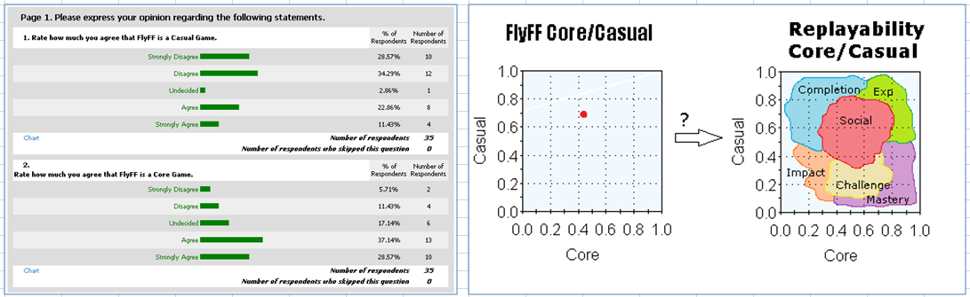
Core Games and Casual Games
No person is entirely a casual or core gamer, nor can you define them as “50% casual, 50% core.” What about games?
Some people have mixed opinions about the nature of the games they love to play. Survey on FlyFF: http://www.esurveyspro.com/Survey.aspx?id=92c00c57-ee20-4047-9ed4-100fae8b7644
From that, perhaps we can assign replayability-aspect importance to different core-casual scores.
Frustration with concept Lattices
I've been trying to implement this:
http://www.gbspublisher.com/ijtacs/1010.pdf
Unfortunately, I just haven't been able to so far. Hopefully have something by the meeting.
http://www.gbspublisher.com/ijtacs/1010.pdf
Unfortunately, I just haven't been able to so far. Hopefully have something by the meeting.
Tuesday, January 10, 2012
Virtual Machine and You: A match made in coding heaven
Here's the link to set up Ubuntu Virtual Machine, you crazy coders you:
From here, go to Projects->Homework 1
E-mail me if you have questions.
Monday, January 9, 2012


Friday, December 16, 2011


Monday, December 5, 2011
unsupervised learning results
nasa93
> ,kloc,0
> ,acap,0.22927988981346761332
> ,data,0.2334438373917348819
> ,time,0.25423355037952316549
> ,plex,0.26866055225810964169
> ,stor,0.27441589382858594393
> ,pmat,0.3093114132807298633
> ,cplx,0.34470954768369121979
> ,apex,0.35198812495229314656
> ,pcap,0.36553252022821636213
> ,rely,0.40329996377433946497
> ,ltex,0.46603801062070232542
> ,pvol,0.56369464132541236001
> ,sced,0.58780717952192207409
> ,tool,0.82277351898917538975
> ,docu,1
> ,flex,1
> ,pcon,1
> ,prec,1
> ,resl,1
> ,ruse,1
> ,site,1
> ,team,1
coc81
> ,tool,0
> ,acap,1
> ,aexp,1
> ,cplx,1
> ,data,1
> ,dev_mode,1
> ,lexp,1
> ,loc,1
> ,modp,1
> ,pcap,1
> ,project_id,1
> ,rely,1
> ,sced,1
> ,stor,1
> ,time,1
> ,turn,1
> ,vexp,1
> ,virt,1
desharnais
>> ,YearEnd,0
>> ,Adjustment,1
>> ,Entities,1
>> ,Langage,1
>> ,Length,1
>> ,ManagerExp,1
>> ,PointsAjust,1
>> ,PointsNonAdjust,1
>> ,Project,1
>> ,TeamExp,1
>> ,Transactions,1
finnish
>> ,prod,0
>> ,at,1
>> ,co,1
>> ,FP,1
>> ,hw,1

nasa93n
>> ,prec,0
>> ,flex,0.11243402160650950439
>> ,docu,0.33052121547798030132
>> ,resl,0.40212091296737206836
>> ,apex,0.46229399349528710328
>> ,data,0.46229399349528710328
>> ,acap,0.61482323785435888386
>> ,pvol,0.61482323785435888386
>> ,sced,0.61482323785435888386
>> ,stor,0.61482323785435888386
>> ,cplx,0.70398054754829086921
>> ,kloc,0.78682242656022605143
>> ,ltex,0.78682242656022605143
>> ,pcap,0.78682242656022605143
>> ,pmat,0.78682242656022605143
>> ,rely,0.78682242656022605143
>> ,ruse,0.78682242656022605143
>> ,team,0.78682242656022605143
>> ,time,0.78682242656022605143
>> ,tool,0.78682242656022605143
>> ,plex,0.87700247550119436735
>> ,site,0.87700247550119436735
>> ,pcon,1

china
>> ,Duration,0
>> ,Resource,0.18076822524622718213
>> ,Enquiry,0.70229300937753547096
>> ,Added,0.70418156239280693676
>> ,NPDR_AFP,0.71748509491228684709
>> ,AFP,0.84023872986505276916
>> ,N_effort,0.84023872986505276916
>> ,Interface,0.85325277904975838084
>> ,File,0.9226111617867434056
>> ,Input,0.94562919153491631352
>> ,Output,0.96948001254205484756
>> ,Changed,0.98391349972332420304
>> ,Deleted,1
>> ,Dev.Type,1
>> ,ID,1
>> ,NPDU_UFP,1
>> ,PDR_AFP,1
>> ,PDR_UFP,1

miyazaki94
>> ,KLOC,0
>> ,FORM,0.40638957366031353002
>> ,ESCRN,0.43471405099857385324
>> ,EFILE,0.63742030743007560556
>> ,FILE,0.74270091796517645477
>> ,EFORM,0.89605538051121036425
>> ,SCRN,1
MRE results
Just listening to the best X percent of attributes, sorted by entropy.#data sets cutoff a ignore 0 25 50 75 100 ---------------- ------ - ------------- --- --- ---- ---- ---- data/nasa93.arff, 0.25, 5, 1, , , 10, 0, |, 0, 0.6, 0.81, 0.91, 9.99 data/nasa93.arff, 0.33, 7, 1, , , 10, 0, |, 0, 0.51, 0.77, 0.89, 7.33 data/nasa93.arff, 0.5, 11, 1, , , 10, 0, |, 0, 0.35, 0.69, 0.85, 33.08 data/nasa93.arff, 0.66, 15, 1, , , 10, 0, |, 0, 0.37, 0.61, 0.84, 7 data/nasa93.arff, 0.75, 23, 1, , , 10, 0, |, 0, 0.4, 0.63, 0.9, 12.5 data/nasa93.arff, 1, 23, 1, , , 10, 0, |, 0, 0.42, 0.63, 0.83, 7.33
data/desharnais.arff, 0.001,  1, 1, , , 10, 0, |, 0, 0.34, 0.46, 0.65, 5.92
data/desharnais.arff,  0.25, 11, 1, , , 10, 0, |, 0, 0.22, 0.37, 0.56, 3.87
data/desharnais.arff,  0.33, 11, 1, , , 10, 0, |, 0, 0.25, 0.37, 0.56, 3.87
data/desharnais.arff,   0.5, 11, 1, , , 10, 0, |, 0, 0.25, 0.37, 0.56, 3.87
data/desharnais.arff,  0.66, 11, 1, , , 10, 0, |, 0, 0.25, 0.37, 0.56, 3.87
data/desharnais.arff,  0.75, 10, 1, , , 10, 0, |, 0, 0.27, 0.48, 0.62, 4.18
data/desharnais.arff,     1, 11, 1, , , 10, 0, |, 0, 0.25, 0.37, 0.56, 3.87
data/finnish.arff, 0.001, 1, 1, , , 10, 0, |, 0.02, 0.48, 0.71, 0.81, 5.23
data/finnish.arff,  0.25, 1, 1, , , 10, 0, |, 0.05, 0.59, 0.79, 0.85, 4.77
data/finnish.arff,  0.33, 1, 1, , , 10, 0, |, 0.01, 0.58, 0.72, 0.84,  4.9
data/finnish.arff,   0.5, 5, 1, , , 10, 0, |, 0.09, 0.61, 0.76, 0.85,  9.5
data/finnish.arff,  0.66, 5, 1, , , 10, 0, |, 0.09, 0.61, 0.76, 0.85,  9.5
data/finnish.arff,  0.75, 5, 1, , , 10, 0, |, 0.09, 0.61, 0.76, 0.85,  9.5
data/finnish.arff,     1, 5, 1, , , 10, 0, |, 0.09, 0.61, 0.76, 0.85,  9.5
data/coc81.arff, 0.001,   , 1, , , 10, 0, |, 0.07, 0.63, 0.82, 0.98, 15.92
data/coc81.arff,  0.25, 18, 1, , , 10, 0, |, 0.04, 0.76, 0.93,    1, 15.25
data/coc81.arff,  0.33, 18, 1, , , 10, 0, |,    0,  0.6, 0.77, 0.93, 18.58
data/coc81.arff,   0.5, 18, 1, , , 10, 0, |, 0.04, 0.63, 0.86, 0.98,  30.5
data/coc81.arff,  0.66, 18, 1, , , 10, 0, |, 0.04, 0.62, 0.89, 0.99, 27.75
data/coc81.arff,  0.75, 18, 1, , , 10, 0, |,    0, 0.49, 0.85, 0.98, 15.92
data/coc81.arff,     1, 18, 1, , , 10, 0, |,    0, 0.63, 0.84, 0.98, 17.47
data/coc81.arff, 0.001,  1, 1, , , 10, 0, |, 0.04, 0.69,  0.9, 0.98, 14.57
data/coc81.arff,  0.25, 18, 1, , , 10, 0, |,    0, 0.47, 0.82, 0.96, 27.75
data/coc81.arff,  0.33, 18, 1, , , 10, 0, |, 0.01, 0.66, 0.86, 0.98, 15.92
data/coc81.arff,   0.5, 18, 1, , , 10, 0, |, 0.04, 0.58, 0.86, 0.98, 16.96
data/coc81.arff,  0.66, 18, 1, , , 10, 0, |, 0.05, 0.62, 0.94, 1.45, 25.86
data/coc81.arff,  0.75, 18, 1, , , 10, 0, |,    0, 0.62, 0.91, 0.96, 15.92
data/coc81.arff,     1, 18, 1, , , 10, 0, |, 0.06, 0.69, 0.88, 0.99, 15.92
data/miyazaki94.arff, 0.001, 1, 1, , , 10, 0, |,    0, 0.24, 0.45,  0.7,  6.02
data/miyazaki94.arff,  0.25, 1, 1, , , 10, 0, |,    0,  0.2, 0.46, 0.76, 14.25
data/miyazaki94.arff,  0.33, 2, 1, , , 10, 0, |, 0.03, 0.39, 0.61, 0.72, 14.25
data/miyazaki94.arff,   0.5, 3, 1, , , 10, 0, |, 0.01, 0.24, 0.43, 0.63,  4.36
data/miyazaki94.arff,  0.66, 4, 1, , , 10, 0, |,    0,  0.4, 0.61, 0.79,  3.79
data/miyazaki94.arff,  0.75, 5, 1, , , 10, 0, |, 0.02, 0.31, 0.45, 0.72,  3.57
data/miyazaki94.arff,     1, 7, 1, , , 10, 0, |,    0,  0.2, 0.63, 0.78,  5.35
data/china.arff, 0.001,  1, 1, , , 10, 0, |, 0,  0.5, 0.76, 0.94, 93.48
data/china.arff,  0.25,  5, 1, , , 10, 0, |, 0, 0.14, 0.27, 0.45, 14.67
data/china.arff,  0.33,  5, 1, , , 10, 0, |, 0, 0.44, 0.66, 0.83, 46.84
data/china.arff,   0.5,  9, 1, , , 10, 0, |, 0, 0.21, 0.37, 0.58,  8.46
data/china.arff,  0.66, 13, 1, , , 10, 0, |, 0, 0.24, 0.38, 0.59, 13.63
data/china.arff,  0.75, 18, 1, , , 10, 0, |, 0, 0.38, 0.58, 0.76, 12.08
data/china.arff,     1, 18, 1, , , 10, 0, |, 0, 0.37, 0.57, 0.75, 19.35

Tuesday, November 29, 2011
Tuning a learner
See http://unbox.org/stuff/var/timm/11/idea/data/ideasMAR_fss.txt for what happens when I run and http://unbox.org/stuff/var/timm/11/idea/html/idea.html to generate http://unbox.org/stuff/var/timm/11/idea/data/ideasMAR.csv, then summarize with http://unbox.org/stuff/var/timm/11/idea/ideas.sh through feature selection
Monday, November 28, 2011
Monday, November 14, 2011


1. Bias Variance Analysis
a) Anova -> Bias is 8/20, Variance is 14/20
b) Scott&Anova -> Bias is 8/20, Variance is 15/20
c) Anova plus Cohen's correction: Bias is 8/20
d) Kruskal-Wallis not so good: Bias is 4/20 and variance is 10/20
e) Sorted bias values of all the data sets plotted are here.
The above plots showed us that there are extreme values due to new experimental conditions.
f) The Friedman-Nemenyi plots are here for separate data sets.
g) The same test as before for the entire 20 data sets together are here.
h) Re-generate boxplots with the new experimental conditions.
I applied a correction on the analysis, because...
Here is the paper with new boxplots..
Here is the Friedman Nimenyi plots on separate data sets, bias is the same for 15 out of 20 data sets..
Below is the result of Friedman Nimenyi over all data sets, i.e. if we see it as 20 repetitions.

2. Papers
a) HK paper is revised and is ready to be seen here.
b) Active learning paper's major revision is submitted to TSE.
c) Camera ready versions of ensemble and kernel papers are submitted to TSE and ESEM.
3. The break-point experiments
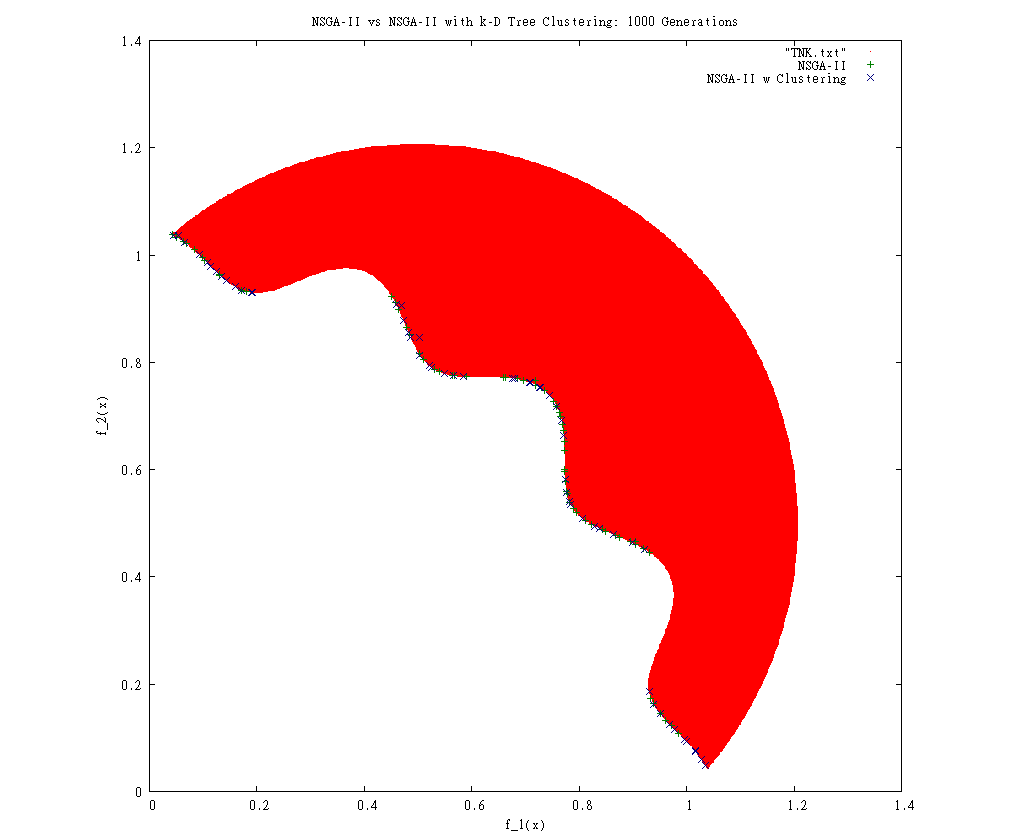
Clustering Accelerates NSGA-II

Using a natural clustering method, and replacing poor solutions with solutions bred within "interesting" clusters, appears to accelerate how quickly NSGA-II converges upon the Pareto frontier with little impact on the diversity of the solutions or the speed of the algorithm.
Clusters are divided by heuristically and recursively dividing space along a natural axis for the individuals. The FastMap heuristic is used to pick individuals that are very distant from each other by their independent attributes. All the other individuals are placed in the coordinate space by the magnitude of their orthogonal projections onto the line between the two extreme individuals. A division point is chosen along this axis that minimizes the weighted variance of the individuals' ranks. The splitting continues on each half of the split down to "sqrt(individuals)".
An "interesting" cluster is one that has at least one first-rank individual within it and a low ratio of first-rank individuals to total individuals in the cluster. A "boring" cluster is either completely saturated with first-rank individuals or lower-ranked individuals.
Tuesday, November 1, 2011
Raw data from hall et al
https://bugcatcher.stca.herts.ac.uk/slr2011/
A Systematic Review of Fault Prediction Performance in Software Engineering
http://www.computer.org/portal/web/csdl/abs/trans/ts/5555/01/tts555501toc.htm
http://ieeexplore.ieee.org/xpls/abs_all.jsp?arnumber=6035727&tag=1
stats methids
divide numbers such that the entropy of the treatments they select is minimal: http://unbox.org/stuff/var/timm/11/id/html/entropy.html
divide performancescores such that the variance t is minimal: http://unbox.org/stuff/var/timm/11/id/html/variance.html
given N  arrays of performance results p .... of treatments 1,2,3...
with means  m[1],m[2], etc
with stand devs of s[1], s[2], etc then ...

for i in N
   for j in N
        boring[i,j] = (abs(m[i] - m[i])/s <= 0.3) #cohen

samples=1000
N*samples timesRepeat: {
   i = any index 1..N
   j= any index 1..N
  if (boring[i,j] continue
   x = the i-th member of p[i]
   y = the j-th member of p[j]
   diff = x - y
   better = if(errorMeasures) diff<0 else diff>0
   win[i] += better
}
for(i in win)
   win[i] = win[i]/(N*samples) * 100 # so now its percents

rank treatments by their position in win (higher rank = more wins)
Monday, October 10, 2011
Reviews and unsupervised feature-selectors
a) Papers: In case you want to take a look at some of the recent reviews we have submitted, here are two papers: 1) kernel density estimation and 2) ensemble methods.
Another one with 40% of the reviews done is about active learning (here).
b) QUICK+ (under implementation): An unsupervised instance and feature selector, which works in two steps:
Another one with 40% of the reviews done is about active learning (here).
b) QUICK+ (under implementation): An unsupervised instance and feature selector, which works in two steps:
- Step1: Run QUICK on the dataset and find how many instances (q) you need.
- Step2:
- For q instances, transpose the dataset and find the popularity of features in a space defined by instances.
- Throw away features from least popular to most popular until there is a statistically significant deterioration in performance.
- Stop when performance drops significantly and put the last-thrown feature back.
NSGA-II with Clustering Results
Clustering appears to be capable of helping NSGA-II converge faster, but it does not appear to do so reliably. For the two easier problems (Schaffer and Fonseca), the clustering version converges in significantly fewer generations than the baseline version. For the harder problems (Kursawe and Tanaka), it appears to have had little impact.
The clustering appears to have no impact on the variance in convergence.
The following are graphs of the convergences of the two NSGA-II versions on the four problems. The left column shows the median performance, and the right shows the 25th and 75th percentile performances.


The following are graphs of the running times for solving the previous problems. The clustering version is linearly slower than the baseline version.


There are some odd blips in some of the running times that seem to be noise. I tested the Tanaka problem with a population size of 2000 for 2000 generations, and I got a very linear result:

The only thing that can determine whether clustering truly helps NSGA-II perform better is a distribution metric. If clustering helps distribute solutions across the Pareto frontier in fewer generations than the baseline, it may be a viable technique even when it provides no benefit for the convergence.
Tuesday, October 4, 2011
The Continuing Adventures of NSGA-II
I have implemented clustering inside the official NSGA-II implementation in C. It seems to converge faster and with more spread than the baseline:


The trick is processing these results to determine whether the apparent convergence is real or not. The only way I know to test the convergence and distribution is to use the Upsilon (average distance to Pareto frontier) and Delta (distances to neighbors weighted by average distances) measures Deb used, but these require knowing the mathematical definition of the Pareto frontier to calculate equally distributed points across it.
To approximate this, I tried writing an incremental search through the problem space using kd-clustering to refine the search space. To my surprise, it did not seem to work well:

So, I've tried switching to use calculus to determine these points by hand. This is not going well, either:
Schaffer Pareto Frontier: f2 = (sqrt(f1) - 2)^ 2
Area under Frontier: Integral fx dx = 1/2 x^2 - 8/3 x sqrt(x) + 4x + C
Calculating x's that generate precise areas... ?
Crowd pruning
Tried 2 methods:
1) Based on the ratio of (max allowed / current rule count), I randomly decide whether to include each point.
2) I sort by the first dimension, then add in in order every nth item to get to 100. (If n is not an integer, it selects every item that makes the "step" go over the next integer value.
Using algorithm one, I saw a fair amount of performance loss, as gaps began to appear in the frontier.

However, when I used the second algorithm, I saw mostly the same level of performance as the data where I didn't crowd prune the rules, and generated the results is minutes rather than a few hours.

For comparison, here's the fonseca curve at generation 9 without rule pruning.

Still reviewing..
Finished the reviews of the Comba paper minor revision for TSE. The paper is here. I still need a proof-read.
Submitted version of the kernel paper to EMSE is here.
Active learning paper major revisions for TSE are in progress..
Discussion on the TSE paper asserting that OLS is the best.
Experiments: 1) unsupervised feature selectors, 2) different ranking methods.
Submitted version of the kernel paper to EMSE is here.
Active learning paper major revisions for TSE are in progress..
Discussion on the TSE paper asserting that OLS is the best.
Experiments: 1) unsupervised feature selectors, 2) different ranking methods.
Tuesday, September 27, 2011
Current Progress of Lisp NSGA-II
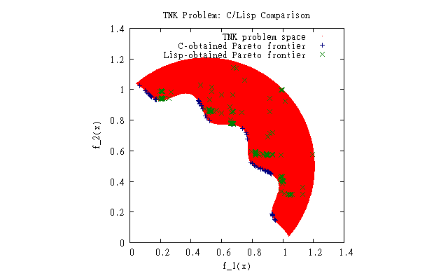 This was the first comparison between the C version and my version. I would have made a new graph, but I somehow lost the C frontier data. I saw that something was very wrong, so I have spent a lot of time trying to fix it. This is as close as I've gotten thus far:
The results are closer, but something is still missing.
Which-2 Function Optimizer Early results
Primarily, we are going to look at the Fonseca data set.
The final curve I was able to generate after 10 generations of running which looks like this:
http://unbox.org/stuff/var/will/frontierfinder/ml/generations/fonseca9.png
It is worth noting that the frontier does not approach f1(x)=0 or f2(x) = 0. Also, on the bottom (leg) of the curve, we see less consistency. This did not seem to improve with future generations.
The overall progression of the generations is here:
http://unbox.org/stuff/var/will/frontierfinder/ml/generations/fonseca1.png
After generation 5, very little seems to change other than a slight change between generations 6 to 9:
http://unbox.org/stuff/var/will/frontierfinder/ml/generations/fonseca.png
Numeric results have not yet been calculated.
Monday, September 26, 2011
Paper Reviews
Tuesday, September 13, 2011
CITRE Data Analysis
Not shockingly, the field that is an order of magnitude larger than the others most affects the data

By comparison, when looking at the other fields, few of the percentages were substantially different from 20% (if, within a class, each of the possible values had a 20% distribution, it would mean true random distribution)
Data (Big file)
Insofar as progress into Which and NSGA-2, I've made progress, though due to illness, not as much as I would like. Hopefully to complete both (or at least 1) by next week with some results.
Monday, September 12, 2011
First Stab at NSGA-2 Optimization
I am working on a modified NSGA-2 to converge on the Pareto frontier in fewer generations than the standard version. My idea is to use clustering to determine the region of independent variable space that is the most promising of those tried in a given generation. By knowing the best spatial region, it should be possible to generate solutions in that region to gain more information than could be gathered breeding initial poor solutions.
My first attempt took a rather simple approach. I made it so that the fast non-dominated sort (FNDS) chose some percentage of the parents for the next generation, and the rest were generated within the most promising space as determined by the above sort. This space was determined by clustering solutions by reducing the standard deviations of the independent variables down to a minimum cluster size of 20, then selecting the cluster that had the lowest mean frontier rank.
This attempt seems to have some promise. Here is a graph showing the baseline performance of the standard NSGA-2 on the Fonseca study:

This is a graph of the two objective scores for all members of the first-ranked frontier for each generation. By generation 20 (far right), NSGA-2 has found a very nice distribution of answers across the Pareto frontier. The first generation that looks close enough to me is generation 14. Note how the first few generations are rather noisy; it isn't until generation 8 that the solutions starts to mostly lie on the Pareto frontier.
As a counterpoint, here is a like graph of my modified NSGA-2. For this run, FNDS selects 80% of the parents, and the remaining 20% are generated from the best cluster:

First, note how the generations converge toward the frontier more rapidly than the baseline. Fewer of the solutions for the initial generations are far away from the Pareto frontier, and by generation 6, the Pareto frontier is outlined almost as strongly as it is in generation 8 from the baseline.
There seem to be diminishing returns from this approach, however. After the baseline NSGA-2 has "discovered" the Pareto frontier, it smoothly converges onto it and distributes solutions across it rather nicely. My modified NSGA-2 seems to be injecting noise that keeps it from converging smoothly across the solution space. This is probably because NSGA-2 is designed to distribute solutions across the Frontier, whereas my current clustering approach searches only one part of it. Furthermore, no adjustments are currently made to account for the algorithm getting closer to the answer, so good solutions are getting replaced by guesses made by the clusterer.
For the next step, I will explore ways to make the clusterer explore all the promising spaces as opposed to just the best one, and also to dynamically adjust the ratio of FSDN-selected parents to cluster-selected parents based upon the proximity to the Pareto frontier.
Wrapping up after the quals
1. ESEM 2011 Talk: Version1 of our presentation is here.
2. The papers waiting for revision are:
2. The papers waiting for revision are:
- Active Learning Paper at TSE (major changes (for 2 goods, 1 excellent) due 5th December 2011)
- Kernel Paper at ESEM (minor changes due 29th September 2011)
- Ranking Stability Paper at ASE (major-awaiting the return from TSE about ensemble paper)
- Bias-Variance Paper (new statistical test)
- Hong-Kong paper (waiting for submission after the reviews of Dr. Keung & Dr. Menzies)
- Find a list of 10+ unsupervised feature selectors
- See this work as a follow-up or complement of the active learning paper, i.e.
- Use the same datasets as the active learning paper
- Run only feature selectors and see which datasets can give the same performance with less features. This will show if it works at all.
- If prior succeeds, then run active learner (with k=1) followed by successful feature selectors. Then change this order and get another run. Compare performance to using the whole dataset and see if feature selection and active learning can complement one another.
- Reading the TSE paper for better understanding
- Formulating the ET test in a formal manner
- Replicating the ASE paper to confirm/refute the ranking changes
- If the previous one succeeds, then building ensembles to see if the ET test outcomes are confirmed by successful multi-methods (???)
Monday, September 5, 2011
Game AI vs Traditional AI
Very recent topic about Traditional AI and Game AI, and what is best for entertainment in games.
http://altdevblogaday.com/2011/07/11/students-game-ai-vs-traditional-ai/
We are still very far behind in terms of "good AI"; Game developers tend to avoid Traditional AI
"Game Developers don't get paid to be clever" - most of the stuff in games today are just tricks, smokes and mirrors, designed to increase believability and make for better games.
The important part is to make a fun and compelling game. Traditional AI takes lots of time and memory, and it doesn't even get used much.
Dungeon Game

Dungeon Game is updated with a simple competitive game play. You need to find the key and then take it to the exit (faster than the Agent.)
We want the Agent to play like a human, so that the game is fair, and as fun as it can be.
The Algorithm powering the Agent is based simply on how I think humans explore. However, data is forthcoming on how humans really explore.
Screenshot: The Agent wins.
Tuesday, August 30, 2011
Results on CITRE from last semester
5 "bands" further examination
ReviewDocs2 = 250
ReviewDocs2 = 275
ReviewDocs2 = 300
ReviewDocs2 = 325
ReviewDocs2 = 350
ReviewDocs2 = 250
ReviewDocs2 = 275
ReviewDocs2 = 300
ReviewDocs2 = 325
ReviewDocs2 = 350
Density Distribution Map

Here is the density distribution map that I came up with for the China Data set. The larger the density, the darker the shade of gray. The pure white spots are where there are no clusters present.
Monday, August 29, 2011
Which2 Multidimensional optimizer
Immediate results using the given multi-dimensional functions are poor, but promising
Fonseca data


Fonseca data

All of our rules with 2-bin discretization using Which were in the tiny green square. However, the goal with fonseca is to minimize, so being in the top right corner is very bad. By comparison, with 8-bin, are rules were mostly in the top right blue square, but we had one rule with coordinates f1=0.2497 f2=0.9575.
In Kursawe

Our rules were all in the mass in the center left when I chose maximize to optimize. With 8-bin, the rules were spread out with than with 2-bin.
This is because 8-bin allows more detail than 2-bin. However, I posit once I am able to recurse this process, applying the constraints of the rules, that 2-bin will be better overall.
Further exploring these rules (by applying the rules as new constraints on the randomized input vectors on the data database) will involve a massive recoding. However, having done some manual constraints using the generated rules, the results improve in Round 2 (treating this as round 1). However, you cannot simply pick one rule to explore. Basically, your unconstrained start point is the head of an infinite tree, the branches from each node are the rules generated by each run of which using that node and all ancestor nodes to that node's rules as constraints on the input data. The rules can then be mapped to coordinates in the space of (f1, f2, ...fn). Ideally, these rules will approach the Pareto frontier.
Which is running through the data very quickly, but until I have further results which will take a massive reworking of code, can't say anything definitive about it's long term usefulness just yet.
Tuesday, August 23, 2011
Privacy Algorithms
4 Privacy algorithms tested against 4 learners (random forests, naive bayes, k-nearest neighbour and logistic regression.
privacy.pdf
privacy.pdf

Fastgrid
This summer I worked on creating a stronger version of idea in lisp. The first code was fastmap which was the 2D point generator. Then instead of storing the data in a tree structure, they were stored in a grid structure. The size and number of quadrantas was determined by the square-root of the amount of the data divided by two. When looking to cluster the quadrants, the gridclus function could take a look at all directions surrounding it to find its' closest neighbors.
Then the neighbors of the neighbors were searched for acceptance rate of 0.5 also. Gaps was then coded to compare clusters and locate the closet neighbor feared by the cluster being looked at. Finally, Keys was created to look for the best treatment. It used (b/B)^2/((b/B) +(r/R)) to determine the best rule overall. b is the frequency the rules appears in the 20% best, while r is the frequency that the rule appears in the 80% rest. While all of these functions were coded up individually, they are not yielding the correct results.
As seen from the image, the grid still contains too many clusters. When taking a closer look, it can be seen tath several of tehse clusters should be mereged t into one. The gridclus error is the start of the problems with the different functions interacting.
This example is from the velocity 1.6 data.

There are 30 clusters with the most in one cluster equally 4 quadrants.
An example of the printout when keys is run on this data follows:
KEYS
(CLUSTER AB)
(ENVIES AL)
(TREATMENT #((0.0 $MOA)))
KEYS
(CLUSTER AL)
(ENVIES AZ)
(TREATMENT #((0.0 $NOC)))
KEYS
(CLUSTER AG)
(ENVIES AB)
(TREATMENT #((0.0 $LCOM)))
Then the neighbors of the neighbors were searched for acceptance rate of 0.5 also. Gaps was then coded to compare clusters and locate the closet neighbor feared by the cluster being looked at. Finally, Keys was created to look for the best treatment. It used (b/B)^2/((b/B) +(r/R)) to determine the best rule overall. b is the frequency the rules appears in the 20% best, while r is the frequency that the rule appears in the 80% rest. While all of these functions were coded up individually, they are not yielding the correct results.
As seen from the image, the grid still contains too many clusters. When taking a closer look, it can be seen tath several of tehse clusters should be mereged t into one. The gridclus error is the start of the problems with the different functions interacting.
This example is from the velocity 1.6 data.
There are 30 clusters with the most in one cluster equally 4 quadrants.
An example of the printout when keys is run on this data follows:
KEYS
(CLUSTER AB)
(ENVIES AL)
(TREATMENT #((0.0 $MOA)))
KEYS
(CLUSTER AL)
(ENVIES AZ)
(TREATMENT #((0.0 $NOC)))
KEYS
(CLUSTER AG)
(ENVIES AB)
(TREATMENT #((0.0 $LCOM)))
Monday, August 22, 2011
Lua Games


Attack of the Robots
- Avoid robots, and as they chase you down, get them to run into each other
Grand Theft Wumpus
- The Wumpus is hiding in Congestion City, but where?
- Use clues to track down his blood trail, and avoid Glow-worm gangs and Police
- Fire your one and only shot at the Wumpus if you think you've got his location tracked down
Evolution
- Watch as animals reproduce while eating and expanding across the game world
- Notice how most animals will remain in the lush jungle; very few wander out across the steppes.
Graphics Engine chosen for development was Lua LOVE: http://love2d.org/
Dungeon Gen & Explorer
Dungeon built based off an algorithm by Jamis Buck:http://blog.kromatyk.fr/wp-content/random-dungeon-design.pdf.

 Left: Regions the agent has explored. Right: The entire dungeon; explored.


The agent doing the exploring is what is interesting in the Dungeon Project - I developed an algorithm on my own in which the agent discovers and uses pathfinding to track down "darkways" - points of interest which the agent wants to go explore. The algorithm marks down all darkways, and chooses the closest one to go explore.
This is a human-way of exploring an unknown dungeon, and it is human because the agent has been restricted in what it knows about the dungeon. For instance, the agent only knows what has been revealed into vision, and it's pathfinding includes only visible regions.
 Left: Regions the agent has explored. Right: The entire dungeon; explored.

Subscribe to:
Posts (Atom)