Kernel Mean Match (KMM) for cross-project defect prediction

Context: cross-project defect prediction

Algorithm: Kernel Mean Match

where  B limits the scope of discrepancy between Pr and Pr′ and esp  ensures that the measure β(x) Pr(x) is close to a probability distribution. 

Data: 5 open source project, process metrics (change data)

performance indicators: AUC, F, Recall, Precision


Experiments:

parameter tuning: B=1,3,5,10,20,50; esp=0.01, 0.1, 0.5, 1, 5, 10.

Naive Bayes (B=5, esp=0.01)

AUC	Acc	F	F_2	Recall	Precision	PF	TestSet	TrainSet
0.6749	0.8517	0.2238	0.1752	0.1531	0.4156	0.0349	PDE_change	JDT_change
0.6731	0.6451	0.2282	0.1586	0.1318	0.8500	0.0154	equinox_change	JDT_change
0.7555	0.9204	0.3529	0.2708	0.2344	0.7143	0.0096	lucene_change	JDT_change
0.6424	0.8598	0.1092	0.0778	0.0653	0.3333	0.0198	mylyn_change	JDT_change
0.7185	0.6229	0.4551	0.6002	0.7621	0.3244	0.4134	JDT_change	PDE_change
0.7953	0.6944	0.4343	0.3381	0.2946	0.8261	0.0410	equinox_change	PDE_change
0.7772	0.8857	0.4060	0.4154	0.4219	0.3913	0.0670	lucene_change	PDE_change
0.5753	0.8448	0.2684	0.2345	0.2163	0.3533	0.0600	mylyn_change	PDE_change
0.7488	0.6810	0.4838	0.6037	0.7233	0.3634	0.3300	JDT_change	equinox_change
0.6985	0.7508	0.3935	0.4871	0.5789	0.2980	0.2213	PDE_change	equinox_change
0.7118	0.7424	0.3101	0.4444	0.6250	0.2062	0.2456	lucene_change	equinox_change
0.5615	0.7873	0.2826	0.3030	0.3184	0.2541	0.1416	mylyn_change	equinox_change
0.7411	0.6911	0.4901	0.6056	0.7184	0.3719	0.3161	JDT_change	lucene_change
0.6889	0.7916	0.3735	0.4133	0.4450	0.3218	0.1522	PDE_change	lucene_change
0.7825	0.7222	0.5588	0.4822	0.4419	0.7600	0.0923	equinox_change	lucene_change
0.6489	0.8281	0.3043	0.2929	0.2857	0.3256	0.0897	mylyn_change	lucene_change
0.6040	0.3400	0.3286	0.5038	0.7816	0.2080	0.7750	JDT_change	mylyn_change
0.5824	0.5311	0.2626	0.3958	0.5981	0.1682	0.4798	PDE_change	mylyn_change
0.5599	0.6636	0.5068	0.4605	0.4341	0.6087	0.1846	equinox_change	mylyn_change
0.6228	0.7829	0.2857	0.3731	0.4688	0.2055	0.1850	lucene_change	mylyn_change

KMM vs. non-weights

B=5 esp=0.01	non-weights
AUC	AUC	improvement	mean(imp)	median(imp)
0.6749	0.6313	0.0436	0.0218	0.0228
0.6731	0.7702	-0.0970
0.7555	0.7149	0.0406
0.6424	0.4153	0.2271
0.7185	0.7207	-0.0022
0.7953	0.7843	0.0110
0.7772	0.7413	0.0359
0.5753	0.5716	0.0038
0.7488	0.7105	0.0384
0.6985	0.6843	0.0142
0.7118	0.7257	-0.0139
0.5615	0.5131	0.0484
0.7411	0.7098	0.0313
0.6889	0.6954	-0.0065
0.7825	0.7739	0.0086
0.6489	0.6140	0.0349
0.6040	0.6305	-0.0265
0.5824	0.6424	-0.0601
0.5599	0.5102	0.0497
0.6228	0.5678	0.0550

Observations:
1) after parameter tuning, KMM helps to improve prediction performance, but not so significant (2%)
2) long running time! 900 training instances + 300 test instances: 30min; 10,000 training instances + 300 test instance: 130 min! 

Questions:
1) KMM may be a stupid idea for cross defect prediction though it's beautiful on mathematics?  


New results(2012-12-18):
parameter tuning: B=1,3,5,10,20,50; esp=0.01, 0.1, 0.5, 1, 5, 10.

Fig. 1 Improvement of PD

Fig. 2. Improvement of PF

POM2 RRSL SPEA2 and NSGAII

Charts: 

http://unbox.org/stuff/var/joe/joe/fall2012/pom2rrslTesting/charts/

RRSL significantly worse than SPEA2 and NSGAII but runtimes and evaluations used are significantly less.  POM2 Idle & Incompletion are not very well controlled, and RRSL does better with these confoundedly.  

Datatable:

http://unbox.org/stuff/var/joe/joe/fall2012/pom2rrslTesting/charts/rrsl_spea2_nsgaii_datatable.txt

POM2 Baselines

Using Inspyred for Python.  (http://pypi.python.org/pypi/inspyred)
May switch to DEAP, since no SPEA2 in Inspyred.  (http://code.google.com/p/deap/)


NSGA2:
table of data: http://justpaste.it/1la9
charts image: http://i.imgur.com/Ceuw8.png

PAES:
table of data: http://justpaste.it/1laa
charts image: http://i.imgur.com/SAl9D.png

NumEvals above are > 10,000
NumEvals below are < 20

RRSL:
tables of data: http://unbox.org/stuff/var/joe/joe/fall2012/pom2rrslTesting/data/

Workshop on Data Analysis Patterns in Software Engineering

http://research.microsoft.com/en-us/events/dapse2013/

DAPSE’13: International Workshop on Data Analysis Patterns in Software Engineering

The workshop has been accepted to the International Conference on Software Engineering. 

 Data science is a skilled art with a steep learning curve. To shorten that learning curve, this workshop will collect best practices in form of data analysis patterns, that is, analyses of data that leads to meaningful conclusions and can be reused for comparable data. 

In the workshop we will compile a catalog of such patterns that will help both experienced and emerging data scientists to better communicate about data analysis. The workshop is intended for anyone interested in how to analyze data correctly and efficiently in a community accepted way.

EXAMPLE of a PATTERN

For illustrative purposes, here’s an example pattern in short and simplified form. For the workshop, we expect the discussion to be more comprehensive. We do welcome both simple and complex analysis patterns.

Pattern name: Contrast Problem:  Determine if there is a difference in one or more properties between twopopulations. Solution:  1. Apply a hypothesis test (student t-test for parametric data, Mann Whitney test for non-parametric test) to check if the property is statistically different between populations. 2. Determine the magnitude of the difference, either through visualization (e.g., boxplot) or when appropriate through mean or median. Discussion:  Either step without the other can be misleading. For large populations, tiny differences might be statistically significant. In contrast for small populations large differences might not be statistically significant. Choosing the wrong hypothesis test is a common mistake. Examples:  For example, at ICSE 2009, Bird et al. used a Mann Whitney test to compare the defect proneness (=the property) between distributed and co-located binaries (=two populations). See Figure 5 in their paper for a sample visualization of the differences between the two population.

The magic tuning problem

Improved Knowledge Acquisition for High-Performance Heuristic Search
J.P. Bekmann and Achim Hoffmann

http://www.ijcai.org/papers/1668.pdf

We present a new incremental knowledge acquisition approach that incrementally improves the performance of a probabilistic search algorithm. The approach addresses the known dif culty of tuning probabilistic search algorithms, such as genetic algorithms or simulated annealing, for a given search problem by the introduction of domain knowledge. We show that our approach is effective for developing heuristic algorithms for dif ficult combinatorial problems by solving benchmarks from the industrially relevant domain of VLSI detailed routing. In this paper we present advanced techniques for improving our knowledge acquisition approach. We also present a novel method that uses domain knowledge for the prioritisation of mutation operators, increasing the GA's ef ciency noticeably.

Some ICSE 2013 papers...

Papers from ICSE 2013:

Process

Not Going to Take This Anymore: Multi-objective Overtime Planning for Software Engineering Projects

Filomena Ferrucci, Mark Harman, Jian Ren, and Federica Sarro

(University of Salerno, Italy; University College London, UK)

NO RESPONSE

Search-Based SE

How to Effectively Use Topic Models for Software Engineering Tasks? An Approach Based on Genetic Algorithms

Annibale Panichella, Bogdan Dit, Rocco Oliveto, Massimiliano Di Penta, Denys Poshyvanyk, and Andrea De Lucia

(University of Salerno, Italy; College of William and Mary, USA; University of Molise, Italy; University of Sannio, Italy)

INFORMATION RETRIEVAL.

GA, single objective.

Search-Based Genetic Optimization for Deployment and Reconfiguration of Software in the Cloud

Sören Frey, Florian Fittkau, and Wilhelm Hasselbring

(Kiel University, Germany)

Problem: cloud deployment options (CDOs)

Simulator CDOSim can evaluate CDOs, e.g., regarding response times and costs.

Three objectives:

1-     cost refer to the total amount of monetary units owed to a cloud provider because of utilizing provided services.

2-     Response times refer to the average response times of the methods that are included in a workload profile.

3-     SLA violations indicate the number of method calls with response times that exceed a given threshold.

  

Custom algorithms based on NSGA-II.

Improvement by 60% over other tools.

Product Lines

Beyond Boolean Product-Line Model Checking: Dealing with Feature Attributes and Multi-features

Maxime Cordy, Pierre-Yves Schobbens, Patrick Heymans, and Axel Legay

(University of Namur, Belgium; INRIA, France)

Still a Verification method.

Multi-features: features that can appear several times in the same product, e.g. processing units.

On the Value of User Preferences in Search-Based Software Engineering: A Case Study in Software Product Lines

Abdel Salam Sayyad, Tim Menzies, and Hany Ammar

(West Virginia University, USA)

Reviewer #1:

 I suggest that the title be more direct in its description of the paper's content (i.e., make clear that the paper's focus is on evaluating the use of MEOAs in the SPL domain).

Reviewer #2:

The paper has a very nice survey of previous work on SBSE and multi objective SBSE that establishes the context in which the contributions of the paper are made. This is effectively a kind of "mini focused literature review” that focusses on previous work on multi objective SBSE. It is a small contribution
in itself.

The claims are very much overstated and need to be toned down. 

You can't say "who" when referring to an algorithm; they are not alive, no matter how "AI" this SBSE stuff might be :-)

Reviewer #3:

This is a very good paper. It reads like a page-turner…

Also quite original and appealing is the idea of reducing the correctness criteria to just another dimension to optimize.

Tukutuku paper

The latest version of the paper, re-worded, re-positioned according to transfer learning viewpoint is here.

Make cross-project defect prediction a successful story: a research roadmap

#Research questions:

1. For the first release of a new project, how can we learn quality prediction models on cross-project data?

Burak proposed to use NN-filter to help cross-project defect prediction and made some promising results (JASE 2010). Now Fayola is also working on this and do it much better (mostly on small size test sets). There are so much worth being further investigated.

1.1 can we  do better on cross-learning performance ? 

      -- some more effective ways to understand the training and test data, like TEAK?

1.2 can we generalize cross-learning strategies to other data?

      -- not only small test sets and static code measures.

1.3 can we make cross-learning algorithms more scalable?

      -- maybe low dimensionality can help?

2. For the following releases, we have to:

2.1 handle the data shift or concept drift problem caused by development environment change to produce better prediction results.

      -- now I'm going on this direction, see my post for last week's group meeting.

2.2 know whether cross-project data can further improve the prediction performance   even though we have local data. If cross-project data works, how should we make use of it?

#Potential solutions:

transductive transfer learning for research question 1, and inductive transfer learning for research question 2.

      -- transductive transfer learning: plenty of  labeled data in the source domain, no labeled data in target domain is available.

      -- inductive transfer learning:  plenty of labeled data in the source domain and a small number of labeled data in the target domain are available.

#My expectation:

1-2 publication on this topic.
     -- FSE conference, JESE, or somewhere better.

All comments are welcome.

Zhimin

Interesting tidbits from Discover Magazine

Nate Silver will tax your crap

Tarnished Silver

Effort Estimation Intrinsic Dimensions

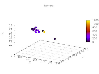
Code to compute the correlation dimension as a function of "r". Note that the intrinsic dimensionality of a data set is, at most, the steepest slopes in a plot of log(C(r)) vs log(r).

@include "lib.awk"
@include "dist.awk"
@include "readcsv.awk"

function _cr(   o) {
  if(args("-d,data/nasa93.csv,-steps,20,-jumps,4",o))
    cr(o["-d"],o["-steps"],o["-jumps"])
}
function cr(f,steps,jumps,
   _Rows,r,k,c,x,logc,logr) {
  readcsv("cat "f,_Rows)
  distances(_Rows,x)
  for(r=1/steps; r<=1 ; r+= 1/steps) {
    c = correlationDimension(r,x,length(d))
    if (c==0) continue
    if (c==1) break
    k++
    print (logr[k] = log(r)) "\t" (logc[k] = log(c)) 
  }
  say("# " steepest(k,jumps,logr,logc)  " " f "\n")
}
function distances(_Rows,x,       i,j) {
  for(i in all)
    for(j in all)
      if (j > i) 
x[i][j] = dist(all[i],all[j],_Rows,1)
}
function correlationDimension(r,x,n,   i,j,c) {
  for(i in x)
    for(j in x[i])
      c += x[i][j] <= r
  return 2/(n*(n-1)) * c
}
function steepest(max,jumps,logr,logc, 
 i,rise,run,m,most) {
  for(i=1; i <= max-jumps; i += jumps) {

    rise = logc[i + jumps] - logc[i]
    run  = logr[i + jumps] - logr[i]
    m    = rise / run
    if (m > most) 
      most = m
  }
  return most
}

And the results are, sorted lowest to highest...

• low
•  0.91  data/china.csv
• 1.97 data/kemerer.csv
• 2.77 data/finnish.csv
• 2.92  data/miyazaki94.csv
• 3.00  data/albrecht.csv
• 3.35 data/nasa93c1.csv
  
  
  
  
  
  
  

• medium
• 3.70 data/coc81o.csv
• 3.96  data/telecom.csv
• 4.00 data/coc81sd.csv
• 4.07  data/coc81.csv
• 4.10 data/desharnais.csv

• high
• 4.51 data/nasa93c2.csv
• 4.54 data/nasa93c5.csv
• 4.78  data/coc81e.csv
• 5.74  data/nasa93.csv
• 8.19  data/sdr.csv

The Peters Filter

The cross-company problem: how to find what train is relevant to you:

Why do cross-company learning?

• Cause when you don't have enough local data, you do very badly
• In the following, we are training and test on very small data sets (lo, median, hi) = 6, 20, 65 instances

So, lets reach out across data sets and compare.

Two cross-company selection filters

• Burak: N things nearest the test data (shown in gray)
• Peters: Cluster the train data, find the clusters with the test data

Note that the Peters  filter uses the structure of the train data to guide the initial selection of the data.

Why?

• Intuition behind Peters' filter: 
• there is more experience in the repo than with you. So use it to guide you

In the following

• Train on selected members of the 46 data sets in the repo (lo, med, hi) = (109, 293,885) instances 
• g = 2*(1 - pf)*pd / (1 - pf + pd) 
• The last column is the delta between peters and burak Filter
• Delta is usually positive and large

The

Does transfer learning work for cross project defect prediction?

The data shift issue  troubles software defect prediction mainly at two aspects:

1) at the time dimensionality: for multi-version projects, historical data of early releases may not applicable for new release.

2) at the space dimensionality: because of the data lack problem, we need to do cross-project defect prediction in some cases.

We see transfer learning as a potential solution to data shift problem of defect prediction for its capability to learn and predict under different training and test distribution.  Our on going experiments support this argument.

First, we observe serious performance reduction on cross-release and cross-project defect prediction (i.e., at the time dimensionality and the space dimensionality ).

Second, after employ a transfer learning framework BDSR (Bias Reduction via Structure Discovery), we do better on cross defect prediction.

--Zhimin 

Novel Subspace Clustering

Novel Subspace Clustering algorithm that uses a top-down FP Growth approach for attribute filtering versus the typically agglomerative bottom-up Apriori paradigm.

It produces disjoint clusters of various dimensionality and does not suffer from the exhaustive subspace search problem of bottom-up approaches.  It finds the densest, correlated attributes and then searches the points for patterns (clusters).

As with most subspace and projected clustering algorithms, the clustering is done in a cyclical manner.  In this method, FP Growth is used to find an candidate attribute subset, then EM clustering is performed over the attributes. EM produces multiple clusters, which are tested by classification learners. Good clusters are labeled and removed from the data set, creating disjoint instance clusters.  The null and bad clusters remain in the data set for further cycles of clustering.  All attributes are available for the FP Growth step and may be repeated in later clusters.

This method requires several parameters, for FP Growth, EM clustering, minimum test and stopping criteria. I believe that it will be significantly less sensitive to the parameter values than current methods. I also believe that it will be more computationally efficient than existing techniques since it uses FP Growth to find candidate subspaces escaping a combinatorial search, and removes clustered instances reducing the overall data set size.

Literature surveys compare the performance of methods over varying data set  sizes.  Moise09 varies attribute size and instance size to create several data sets, but does not test against data sets with roughly the same attribute and instance size.  My method was designed for this case, named the n x m problem. Other subspace and projected clustering algorithms suffer as the attributes are increased; whereas my method is suited to scalability.

- Erin

Intrinsic dimensionality

Here's an article playing my song:

http://www.stat.berkeley.edu/~bickel/mldim.pdf (cited by 300+ people)

Maximum Likelihood Estimation of Intrinsic Dimension
Elizaveta Levina
Peter J. Bickel

In Advances in NIPS, volume 17. MIT Press, 2005
There is a consensus in the high-dimensional data analysis community that the only
reason any methods work in very high dimensions is that, in fact, the data are not
truly high-dimensional. Rather, they are embedded in a high-dimensional space,
but can be e±ciently summarized in a space of a much lower dimension, such as a
nonlinear manifold. Then one can reduce dimension without losing much informa-
tion for many types of real-life high-dimensional data, such as images, and avoid
many of the \curses of dimensionality".

Most standard method: the correlation dimension plot log(C(r)) vs log(r):

They go on to offer another method, which I don't understand, but the resulting numbers are very close to (1).

For a sample of these log(C(r)) vs log(r) graphs, see fig1 of http://oldweb.ct.infn.it/~rapis/corso-fsc2/grassberger-procaccia-prl1983.pdf

Looking at the data

These figures are  hypercube projections of effort data sets.

The first side was picked at random and runs between any two corners 0,1.

After than, side N=2,3,4... was built by picking a point whose sum of the distances to  corners 0,1,...N-1 is maximal.