Intrinsic Dimensionality Baseline

New graph: The effect of (dataset length / critical length) on results. This was done at Q=0.7 and Rmax=len(R)/16. Shown here with 2, 3, 4, and 5 dim random data.

Some more progress on the paper: latest pdf

Consolidated some of my code... relevant files: 

• numberic_fab_and_test.py
• effort.py
• utils.py

Results from revised SE effort data:

Simple stuff first. here's some terrible results from high-dimension random sets:

I had some problems with finding a good slope value for small datasets. The solution I found was the median of two-point slopes to a point. This seems to yield good results in places where the finite slope failed (see below).

Unique IDs crater ID. See Miyazaki94 and my modified Miyazaki2:

Things like dates, test fields which represent comments or notes also do nasty things. The effects of this are still visible in some of the effort datasets. I'll need to re-format the by hand to make sure it's well-conditioned if more accurate results are desired.

While staring at these graphs, I realized:

• We're seeing a spectrum of ID from extremely local to extremely global. 
• The local data isn't particularly useful because you're getting an average value of all localities rather than information about a specific locality.
• The global data isn't particularly useful because as r -> max; D -> 0 (a single point)

But what if you were to ignore the summation across all points and focus instead on distances from a single point (say a cluster centroid):

• At the low end, the dimensionality of the cluster would be represented
• As r reaches the edge of the cluster, if there are other nearby clusters, the changes in D will likely be small. If there are no other clusters nearby, D will approach zero until other clusters are reached
• This could potentially be used to select a scale for visualizations or cross-project learning. (If you're going to use a 2-d map, find a subset of points with an ID close to 2.0 to maximize the amount of information conveyed.)
• This might not work, but seems intuitive. I'll do a few conceptual tests for next week.

I also made some progress on certifying results. Smith88Intrinsic derives this relation for the minimum number of test points to show dimensionality M at range R=rmax/rmin with quality Q:

At first, the results were wild. Nmin went through the roof. By restricting R (lowering the maximum value of r which is being used to determine the ID), the ID becomes more representative of the local area and Nmin becomes reduced. (you're not making a statistical claim about as large of a sphere of influence) I set this up as a after-the fact certification envelope check on the figures. After limiting rmax to the 6.25th ptile of all distances and setting Q to 50%, the results look good (N/Nmin > 1) on most things except the effort sets that I need to re-format. If a tighter certification is needed, additional options such as tuning the parameters on a dataset-by-dataset basis is possible.




Results from Brian's Data:
note: the Lymphography dataset is not present because is not available for public download due to private data.

ecoli.csv :: 3.27
glass.csv :: 0.75
hepatitis.csv :: 2.45
iris.csv :: 1.11
labor-negotiations.csv :: 0.68



Intrinsic Dimensionality Results:

ant-1.3.csv :: 3.40

ant-1.4.csv :: 3.61

ant-1.5.csv :: 2.26

ant-1.6.csv :: 2.69

ant-1.7.csv :: 2.08

ivy-1.1.csv :: 1.74

ivy-1.4.csv :: 2.67

ivy-2.0.csv :: 2.21

jedit-3.2.csv :: 2.04

jedit-4.0.csv :: 1.72

jedit-4.1.csv :: 2.03

jedit-4.2.csv :: 2.22

jedit-4.3.csv :: 2.01

log4j-1.0.csv :: 1.95

log4j-1.1.csv :: 2.67

bad file: ././arff/.svn

ant-1.7.arff :: 2.08

camel-1.0.arff :: 2.41

camel-1.2.arff :: 1.98

camel-1.4.arff :: 2.17

camel-1.6.arff :: 2.16

ivy-1.1.arff :: 1.74

ivy-1.4.arff :: 2.67

ivy-2.0.arff :: 2.21

ivy-2.0.csv :: 2.21

jedit-3.2.arff :: 2.04

jedit-4.0.arff :: 1.72

jedit-4.1.arff :: 2.03

jedit-4.2.arff :: 2.22

jedit-4.3.arff :: 2.01

kc2.arff :: 0.01

log4j-1.0.arff :: 1.95

log4j-1.1.arff :: 2.67

log4j-1.2.arff :: 2.12

lucene-2.0.arff :: 2.14

lucene-2.2.arff :: 2.69

lucene-2.4.arff :: 2.94

mc2.arff :: 1.13

pbeans2.arff :: 1.82

poi-2.0.arff :: 1.75

poi-2.5.arff :: 1.13

poi-3.0.arff :: 1.45

prop-6.arff :: 1.83

redaktor.arff :: 2.02

serapion.arff :: 0.32

skarbonka.arff :: 0.66

synapse-1.2.arff :: 1.89

tomcat.arff :: 2.76

tomcattomcat.arff :: 2.76

bad file: ././arff/too_big

velocity-1.5.arff :: 2.12

velocity-1.6.arff :: 3.00

xalan-2.6.arff :: 1.90

xalan-2.7.arff :: 1.96

xerces-1.2.arff :: 2.18

xerces-1.3.arff :: 0.00

xerces-1.4.arff :: 0.01

zuzel.arff :: 1.54

Space Dim | Mean Dimensionality | SD

    5     |         4.60        |  0.10

   10     |         8.37        |  0.20

   15     |         11.34        |  0.13

   20     |         14.64        |  0.26

   25     |         16.99        |  0.26

   30     |         19.30        |  1.08

   35     |         22.32        |  0.58

   40     |         23.71        |  0.72

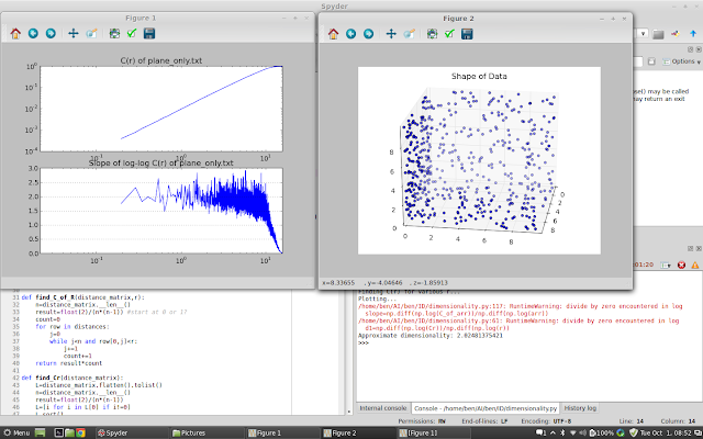
Axes only

Axial Planes only

Random dataset dimensionality vs sparsity and prediction

80% Sparse 3D Dataset

Numeric 3D Dataset

Numberic 10D Dataset

Numberic 100D Dataset

UPDATE 2: PITS vs Randomized:

Original and Word-Randomized Sets of Various Length

Original Data, Word-Randomized with Original Distribution, Word-Randomized with Uniform Distribution

Original Data, Randomized with Original Wordcount Distribution, Randomized with Flat Wordcount Distribution 

Original, Randomized with Original Wordcount dist, Randomized with Gamma Wordcount dist

Original and Randomized with Gamma dist Wordcounts at various Alpha

Original and Randomized with Gamma dist Wordcounts at various Beta

UPDATE: PITS Data:

Cube of uniform distributuion (3-D):

Line of uniform distributuion (1-D):

Spiral of uniform distributuion (1-D):

Plane of uniform distributuion (2-D):

Roling Plane of uniform distribution (2-D):

Line with noise in 1-D, 2-D (line is of length 10, noise is Gaussian SD=0.1):

The Unified Approach paper

SPLOT & LVAT models, IBEA vs. NSGA-II, all the best strategies.

Extending 3 papers: ICSE’13, CMSBSE’13, and ASE’13.

	SPLOT	LVAT	Unified approach
	20 models	7 models	More models?
	43 – 290 features	544 – 6888 features
Continuous dominance vs. Boolean dominance	7 algorithms (ICSE’13) 5 algorithms (TSE)	2 algorithms (ASE’13)	5 algorithms
Best parameters	Pop = 50, crossover = 0, mutation = 0.5/FEATURES (RESER’13)	Pop = 300, crossover = 0.05, mutation = 0.001 (not thoroughly tested)	??
Tree Mutation	TSE	ASE’13 (feature fixing)	Argue that they’re almost the same
Give more weight to constraint satisfaction (8 objectives)			Run 5-obj vs. 8-obj for all 27 models.

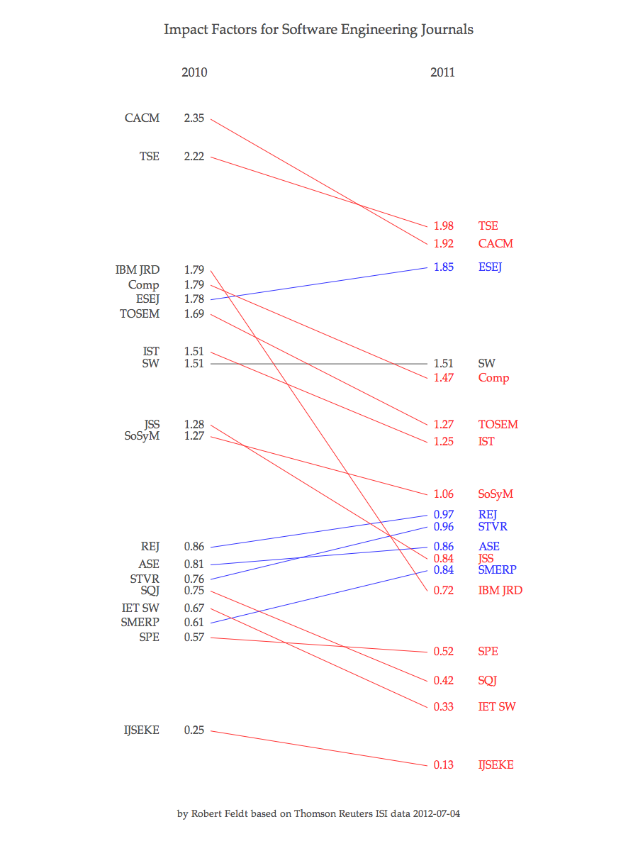
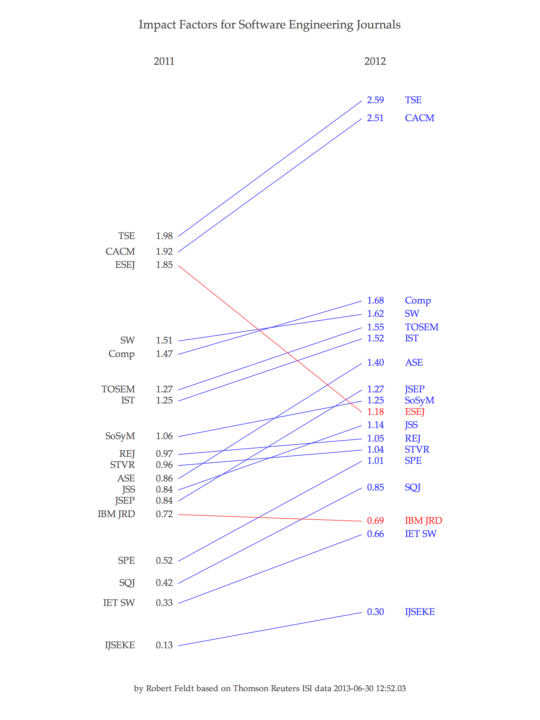
Patterns in academic journals

Source: ISI listed SE journals

2010 to 2011: Houston we have a problem. Falling citation rates on all top journals (except ESEJ)

2011-2012: the reverse trend. All citation counts up (except for ESEJ). And 2 top journals have more citations that before.

Learning Project Management Decisions: A Case Study with Case-Based Reasoning Versus Data Farming

Accepted to TSE

Tim Menzies Adam Brady, Jacky Keung
Jairus Hihn, Steven Williams, Oussama El-Rawas
Phillip Green, Barry Boehm

Download 485K pdf

Abstract

• BACKGROUND: Given information on just a few prior projects, how to learn best and fewest changes for current projects?
• AIM: To conduct a case study comparing two ways to recommend project changes. (1) Data farmers use Monte Carlo sampling to survey and summarize the space of possible outcomes. (2) Case-Based Reasoners (CBR) explore the neighborhood around test instances.
• METHOD: We applied a state-of-the data farmer (SEESAW) and a CBR tool (W2) to software project data.
• RESULTS: CBR with W2 was more effective than SEESAW’s data farming for learning best and recommend project changes, effectively reduces runtime, effort and defects. Further, CBR with W2 was comparably easier to build, maintain, and apply in novel domains especially on noisy data sets.
• CONCLUSION: Use CBR tools like W2 when data is scarce or noisy or when project data can not be expressed in the required form of a data farmer.
• FUTURE WORK: This study applied our own CBR tool to several small data sets. Future work could apply other CBR tools and data farmers to other data (perhaps to explore other goals such as, say, minimizing maintenance effort).

Introduction

In the age of Big Data and cloud computing, it is tempting to tackle problems using:

• A data-intensive Google-style collection of gigabytes of data; or, when that data is missing ...
• A CPU-intensive data farming analysis; i.e. Monte Carlo sampling [1] to survey and summarize the space of possible outcomes (for details on data farming, see §2).

For example, consider a software project manager trying to

• Reduce project defects in the delivered software;
• •Reduce project development effort

How can a manager find and assess different ways to address these goals? It may not be possible to answer this question via data-intensive methods. Such data is inherently hard to access. For example, as discussed in §2.2, we may never have access to large amounts of software process data.

As to the cpu-intensive approaches, we have been exploring data farming for a decade [2] and, more recently, cloud computing. Experience shows that cpu-intensive methods may not be appropriate for all kinds of problems and may introduce spurious correlation under certain situations.
In this paper, we document that experience. The experiments of this paper benchmark our SEESAW data farming tool proposed in against a lightweight case-based reasoner (CBR) called W2.

If we over-analyze scarce data (such as  software process data) then we run into the risk of drawing conclusions based on insufficient background supporting data. Such conclusions will perform poorly on future examples.  For example, from the following data we might generate the RHS blanket. But note we'd be standing on thin ice if we move away from the densest region of the training data.



Our experience shows that the SEESAW data farming tool suffers from many “optimization failures” where if some test set is treated with SEESAW’s recommendations, then some aspect of that treated data actually gets worse. On the contrary W2 has far fewer optimization failures.

So this is like an "anti-MOEA" paper. Algorithms are great but if they over-extrapolate the data, they just produce crap.

Based on those experiments, this paper will conclude that when reasoning about changes to software projects:

1. Use data farming in data rich-domains (e.g. when rea- soning about thousands of inspection reports on millions of lines of code [15]) and when the data is not noisy and when the software project data can be expressed in the same form as the model inputs;
2. Otherwise, use CBR methods such as our W2 tool.

Back story

This paper took four years to complete. In 2009, I was visiting Jacky Keung in Sydney. At that time I was all excited by SEESAW, a model-based data farming tool based on some software process models from USC (COCOMO, etc). Jacky was an instance-based reasoning guy and, as a what-if, I speculated how to do something like SEESAW without COCOMO.

A few months later, I was staying in Naples Florida for a few days and my fingers strayed to a keyboard to try the CBR thing. Took a few hours but the result was "W" ("W" was short for the decider- which is an old joke about the then president at that time) .

W0 [13] was a initial quick proof-of-concept prototype that performed no better than a traditional simulated annealing (SA) algorithm. W1 [14] improved W0’s ranking scheme with a Bayesian method. With this improvement, W1 performed at least as well as a state-of the art model-based method (the SEESAW algorithm discussed below). W2 improved W1’s method for selecting related examples. With that change, W2 now out- performs state-of-the art model-based methods.

• [13] A. Brady, T. Menzies, O. El-Rawas, E. Kocaguneli, and J. Keung, “Case-based reasoning for reducing software development effort,” Journal of Software Engineering and Applications, December 2010.
• [14] A. Brady and T. Menzies, “Case-based reasoning vs parametric models for software quality optimization,” in PROMISE ’10, 2010, pp. 1–10.

The paper was initially rejected, based on some incorrect reviewer conclusions due to some poor writing on my paper. So that delayed the paper 15 months. So lesson one is "stay with it, you'll get there in the end".

Conversations with Deb

Thanks to Marouane Kessentini,  I had time Friday in a Skype meeting with Kalyanmoy Deb of NSGA-II fame.

Deb told me of a new speciality  in optimization. Multi-objective optimization fails for high objective spaces, at which point we go from...

• multi-objective to
• many-objective

Standard many-objective techniques are to (e.g.) 

• learn correlations between objectives to reduce N objectives to M
• use some domain knowledge to find combinations of objectives

Deb has been building NSGA-III that uses "aspiration points" (supplied by the users) for many-objective problems (e.g. a 14 goal objective problem for land usage in New Zealand).  NSGA-III has methods for recognizing  unpractical aspirations then moving them to more achievable aspirations near the Pareto frontier. e.g. http://link.springer.com/chapter/10.1007%2F978-3-642-37140-0_25

Other things said in that meeting:

• HV is ungood for high-objective problems (computational expensive to compute)
• Spread is also ungood in high objective space - diversity is kinda irrelevant in high objective space since the space between the aspiration points can be vast.
• When users state multi-objectives, they often disagree on those objectives. So a real many-objective optimizer has to recognize diversity and clusters of objectives that might be mutual exclusive.

Afterwards, I was thinking:

• about Abdel's stuff- is it really an aspirational-based system?
• about Joe's stuff: if we FASTMAPed on objective space, would we be able to handle higher objective dimensionality?

Anyway, some references on many-objective optimization:

• Evolutionary many-objective optimization: A short review
• A Simulated Annealing-Based Multiobjective Optimization Algorithm: AMOSA

Yet another data mining toolkit

AUK

https://github.com/timm/auk/tree/v0


eg. Naive Bayes classifier. Finds class with highest liklihood

function likelihood(row,total,hypotheses,l,_Tables,k,m,
      like,h,nh,prior,tmp,c,x,y,best) {
   like  = NINF ;    # smaller than any log
   total = total + k * length(hypotheses)
   for(h in hypotheses) {   
      nh    = length(datas[h])
      prior = (nh+k)/total
      tmp   = log(prior)
      for(c in terms[h]) {
         x = row[c]
         if (x == "?") continue
         y = counts[h][c][x] 
         tmp += log((y + m*prior) / (nh + m))
      }
      for(c in nums[h]) {
         x = row[c]
         if (x == "?") continue
          y = norm(x, mus[h][c], sds[h][c])
          tmp += log(y)
      }
      l[h] = tmp
      if ( tmp >= like ) {like = tmp; best=h}
   }
   return best
}

Lit review on transfer learning

Transfer Learning for Software Engineering:
A Literature Review

Tim Menzies, Fayola Peters 
Lane Department of CS & EE, WVU, USA

Forrest Shull, Lucas Layman
Fraunhofer Center for Experimental SE, College Park, MD, USA

tim@menzies.us,
fayolapeters@gmail.com {
fshull,llayman}@fc-md.umd.edu

For decades, empirical methods in SE have focused on a mostly manual analysis of project data. That approach has often suffered from lack of transfer since it was hard to migrate lessons learned from one project to another.

Recently, there has been much success with automatic transfer learning between SE projects. This short paper reviews that work to observe that (1) transfer learning has been far more successful at transferring lessons learned than traditional SE methods; (2) past research on transfer learning has uncovered numerous issues and open issues that need exploring.

Download (380K, pdf)

Two articles in TSE

WVU grad students rule

A Summer in Rear-view - Joe

NASA Ames Report:

In progress of developing a framework for NextGen aviation technology studies.  This framework will investigate the integration of highly-necessary NextGen technology into current aviation policies.

Poster: https://www.dropbox.com/s/rghtyrqvgftqowk/nasa_poster_joe.pdf
Abstract: https://www.dropbox.com/s/71agln6id5h6otw/nasa_poster_abstract_joe.pdf

modeling for optimization:

Objectives:
[min] false alarm rate
[min] distance travelled
[max] granularity
[min] look-ahead time
[min] safe spacing distance
[min] crashes
[min] conflicts

Decisions:
num planes
homogeneous airspace {true, false}   /    num types of planes
num runways
percentage RNP
granularity
look-ahead time
safe spacing distance
[psych] scenario level {SC1, SC2, SC3, SC4, SC5}
[psych] function allocation {FA1, FA2, FA3, FA4, FA5}
[psych] cognitive control model     {OPP, STR, TAC}

California Trip:

In addition to visiting NASA Ames campus, I've visited several other sites as well:
 - Google
 - Stanford
 - Vegas
 - Los Angeles
 - San Francisco
 - Golden Gate Bridge
 - Napa Valley Area

GALE Paper Preview:

http://unbox.org/things/var/joe/active/active-v5.pdf

[culture] [crit] [crit mod] [init kn] [inter-D] [dyna] [size] [plan] [team size]

"New" Decision Bin Charts GALE vs NSGA-II:
POM3A&B: http://i.imgur.com/0CjGLwt.png
POM3C&D: http://i.imgur.com/sCmBrim.png

Sans Completion:
http://i.imgur.com/KrvGfA5.png   {(just look at the stuff on the left)}

Looking Ahead:

Before end of 2013:
- Finish NASA Aviation Project
- "Upgrade" GALE into GALE2.  That means identify current quirks with GALE1 and clean them out to enhance performance.
- Integrate NASA project into GALE2 for testing.

Spring 2014: 
- Finish Ph.D.

GUI Progress

I've come down with strep throat, and I won't be able to make it in today.

There have been a few bug fixes, as well as changing the centroid selection. The user clicks on the graph and a new box will appear overlapping the selected centroid (there will be a better indicator later. It's a placeholder for now).

A new window will be launched so that there will be proper room to see the deltas. Only deltas that are above a threshold will be visible.

I still need to work out bugs, and change it so that the user can pick the threshold. I also intend on adding the ability to see the attributes of a single centroid, as well as making the color of a point on the graph variable to reflect the defect class

This weeks progress - Erin

I still have pneumonia, so I am not attending the meeting.

Prelic match score compares the rows in each bicluster to all other biclusters from the competing biclustering solution, and keeps the highest match score.  This is done for all of the clusters in the first biclustering solution.

The match score for all of the biclusters are averaged to give a final score.

I have the match score implemented and ran it to compare all of the algorithms solutions.
I do not have the analysis of these numbers complete.
I plan on running Wilcoxon against the population of match scores to see if there is a statistical difference between the scores.

I will add in the Jaccard Index and Liu's index to the code to provide additional match measurements. I will also compute Hedges' g for effect size.

Peeker GUI Progress

 Your Centroid Selection Method May Vary

Code 'n Stuff:


Centroid data:

clusterId, x, y, class, lcom3, ce, rfc, cbm, loc
0, 1.58397211319, -0.0432681148317, 0.914285714286, 5, 1, 1, 2, 1
1, 2.58774373831, 0.471971285372, 1.0, 5, 1, 1, 2, 1
2, 1.16517561376, -0.371146048932, 0.432432432432, 5, 1, 1, 1, 1
3, 2.08134724468, 0.182633950752, 0.758620689655, 5, 1, 1, 2, 1
4, 3.07060918722, 0.803626419167, 0.903225806452, 4, 1, 2, 2, 1
5, 2.55082940399, 0.261739913349, 0.75, 5, 1, 1, 2, 1
6, 2.16558214132, 0.480240059556, 0.833333333333, 5, 1, 1, 1, 1
7, 1.29619823833, -0.111457622989, 0.714285714286, 6, 1, 1, 1, 1
8, 1.63873965905, -0.305464834941, 0.285714285714, 3, 1, 1, 1, 1
9, 0.357360583273, -0.912243253683, 0.212121212121, 7, 1, 1, 1, 1
10, 3.20012449807, 0.433418626026, 0.833333333333, 4, 1, 1, 2, 1
11, 3.53375557599, 0.919199863541, 1.0, 5, 1, 2, 2, 1
12, 3.99132169835, 1.5743692604, 0.866666666667, 5, 2, 4, 3, 2
13, 3.17288399009, 1.35969003729, 0.777777777778, 4, 2, 3, 1, 1
14, 2.4873847976, 0.827375341413, 0.777777777778, 4, 1, 2, 2, 1
15, 0.87040871737, -0.342411732755, 0.153846153846, 6, 1, 1, 1, 1
16, -0.477507070513, -1.07814368133, 0.2, 9, 1, 1, 1, 1
17, 1.3265291435, -0.931907015429, 0.230769230769, 5, 1, 1, 1, 1
18, -1.8907652395, -2.92230373138, 0.228571428571, 10, 1, 1, 0, 1
19, 1.67894614243, 0.0792276010178, 0.909090909091, 4, 1, 1, 2, 1
20, 0.363484115168, -1.4811137624, 0.555555555556, 7, 1, 1, 0, 1
21, 2.31618438716, -0.238127701786, 0.434782608696, 5, 1, 1, 1, 1
Code:

from SimPy.SimPlot import *
from ScrolledText import ScrolledText
from tkFileDialog import askopenfilename
import fileinput

plt = SimPlot()
root = plt.root

class TopLevel:
    def __init__(self, root):
        self.filename = StringVar()
       
        self.fileSelect = Menu(root)
        self.fileSelect.add_command(label="Open", command=self.getFile)
        root.config(menu=self.fileSelect)
       
        self.header = Frame(root, width=500, height=20)
        self.topFrame = Frame(root, width=500, height=200, bg="green")
        self.botLeftFrame = Frame(root, width=250, height=200, bg="orange")
        self.botRightFrame = Frame(root, width=250, height=200, bg="yellow")
        self.giveCentroids = Button(root, text="Compare Selected Centroids", command=self.giveCentroids)
       
        self.giveCentroids.grid(columnspan=2,column=0, row=2)
        self.header.grid(columnspan=2, column=0, row=0)
        self.topFrame.grid(columnspan=2, column=0, row=1)
        self.botLeftFrame.grid(column=0, row=3)
        self.botRightFrame.grid(column=1, row=3)
       
        self.grid = Grid(self.topFrame)
        self.list = List(self.botLeftFrame)
        self.compare = Compare(self.botRightFrame)

        self.fDisplay = Label(self.header, textvariable=self.filename)
        self.fDisplay.pack()

    def getFile(self):
        self.filename.set(askopenfilename())
        self.fDisplay.update()
        self.parseFile()
        self.list.setInitialList(self.centroids)
        self.grid.drawGraph(self.centroids)
       

    def parseFile(self):
        # retrieves data points from file. returns list of centroid list of attributes
        for line in open(self.filename.get()):
            if(line[0]=="c"):
                continue
            centroid = []
            for a in line.strip().split(", "):
                centroid.append(a)
            self.centroids.append(centroid)
        # Centroid element: numeric identifier, x, y, defect class, {attributes}
        # print self.centroids
        return self.centroids

    def giveCentroids(self):
        if(len(self.list.selectedCentroids)==2):
            self.compare.giveCentroids(self.list.selectedCentroids)
   
    centroids = []
   
   
class Grid:
    centroids = []
    defectivePoints = []
    nonDefectivePoints = []
   
    def __init__(self, frame):
        self.frame = frame
        self.graph = plt.makeGraphBase(frame, 500, 200)
        self.graph.pack()

    def drawGraph(self, centroids):
        for c in centroids:
            if float(c[3])<.5:
                self.nonDefectivePoints.append([float(c[1]),float(c[2])])
            else:
                self.defectivePoints.append([float(c[1]),float(c[2])])
        self.noDefectSymbols = plt.makeSymbols(self.nonDefectivePoints, marker="square", size=1,fillcolor="blue")
        self.defectSymbols = plt.makeSymbols(self.defectivePoints, marker="square", size=1, fillcolor="red")
        self.obj = plt.makeGraphObjects([self.noDefectSymbols, self.defectSymbols])
        self.graph.draw(self.obj)
       

class List:
    curCentroids = [] #Displayed centroids
    selectedCentroids = [] #Centroids that have been picked
   
    def __init__(self, frame):
        self.frame = frame
       
        self.firstLabel = StringVar()
        self.firstVar = IntVar()
        self.firstCheck = Checkbutton(self.frame, textvariable=self.firstLabel,
                                      variable=self.firstVar, command=self.selectFirstCentroid)
        self.firstCheck.grid(columnspan=2, column=0, row=1)

        self.secondLabel = StringVar()
        self.secondVar = IntVar()
        self.secondCheck = Checkbutton(self.frame, textvariable=self.secondLabel,
                                       variable=self.secondVar, command=self.selectSecondCentroid)
        self.secondCheck.grid(columnspan=2, column=0, row=2)
       
        self.thirdLabel = StringVar()
        self.thirdVar = IntVar()
        self.thirdCheck = Checkbutton(self.frame, textvariable=self.thirdLabel,
                                      variable=self.thirdVar, command=self.selectThirdCentroid)
        self.thirdCheck.grid(columnspan=2, column=0, row=3)

        self.fourthLabel = StringVar()
        self.fourthVar = IntVar()
        self.fourthCheck = Checkbutton(self.frame, textvariable=self.fourthLabel,
                                       variable=self.fourthVar, command=self.selectFourthCentroid)
        self.fourthCheck.grid(columnspan=2, column=0, row=4)
       
        self.prevButton = Button(self.frame, text="Previous", command=self.setPrevList)
        self.nextButton = Button(self.frame, text="Next", command=self.setNextList)
        Label(self.frame, text="Select Centroids").grid(columnspan=2, column=0, row=0)
        self.prevButton.grid(column=0, row=5)
        self.nextButton.grid(column=1, row=5)

    def setInitialList(self, centroids):
        self.centroids = centroids
        for i in range(0,4):
            self.curCentroids.append(centroids[i])
        self.firstLabel.set(self.curCentroids[0][0])
        self.secondLabel.set(self.curCentroids[1][0])
        self.thirdLabel.set(self.curCentroids[2][0])
        self.fourthLabel.set(self.curCentroids[3][0])

    def updateList(self):
        self.firstCheck.update()
        self.secondCheck.update()
        self.thirdCheck.update()
        self.fourthCheck.update()
   
    def setPrevList(self):
        print "filler"

    def setNextList(self):
        print "filler"

    #So I can't get it to pass the relevant centroid. So I need a bunch of functions.
    def selectFirstCentroid(self):
        if len(self.selectedCentroids)>=2:
            self.firstCheck.deselect()
            return
        for i in range(0, len(self.selectedCentroids)):
            if self.curCentroids[0][0]==self.selectedCentroids[i][0]:
                self.firstCheck.deselct()
                return
        # If we're here, we know there aren't too many and the thing isn't already selected
        self.selectedCentroids.append(self.curCentroids[0])

    def selectSecondCentroid(self):
        if len(self.selectedCentroids)>=2:
            self.secondCheck.deselect()
            return
        for i in range(0, len(self.selectedCentroids)):
            if self.curCentroids[1][0]==self.selectedCentroids[i][0]:
                self.secondCheck.deselect()
                return
        self.selectedCentroids.append(self.curCentroids[1])

    def selectThirdCentroid(self):
        if len(self.selectedCentroids)>=2:
            self.thirdCheck.deselect()
            return
        for i in range(0, len(self.selectedCentroids)):
            if self.curCentroids[2][0]==self.selectedCentroids[i][0]:
                self.thirdCheck.deselect()
                return
        self.selectedCentroids.append(self.curCentroids[2])

    def selectFourthCentroid(self):
        if len(self.selectedCentroids)>=2:
            self.fourthCheck.deselect()
            return
        for i in range(0, len(self.selectedCentroids)):
            if self.curCentroids[3][0]==self.selectedCentroids[i][0]:
                self.fourthCheck.deselect()
                return
        self.selectedCentroids.append(self.curCentroids[3])
       
class Compare:
    centroid1 = []
    centroid2 = []
   
    def __init__(self, frame):
        self.frame = frame
        self.display = ScrolledText(frame, width=25, height=7)
        self.display['font'] = ('consolas', '12')
        self.display.pack()
        self.display.insert(END, "Attributes Deltas\n")
        self.display.config(state=DISABLED)

    def giveCentroids(self, centroids):
        self.centroid1 = centroids[0]
        self.centroid2 = centroids[1]
        self.displayDelta()

    def displayDelta(self):
        self.display.config(state=NORMAL)
        for i in range(1,len(self.centroid1)):
            printed = float(self.centroid1[i])-float(self.centroid2[i])
            self.display.insert(END, format(printed)+"\n")
        self.display.config(state=DISABLED)

window=TopLevel(root)

root.mainloop()

Python Development

Retrieving/parsing data from a (junk) file, posting it to a graph(canvas)