Tuesday, November 19, 2013

Version Tracking Visualization

Results 1/21/14


Results of A/B/C/D prediction: dismal


Results 2:


Back to the CSV: class names are listed

['ant-1.3.csv', 'ant-1.4.csv', 'ant-1.5.csv', 'ant-1.6.csv', 'ant-1.7.csv']
Type A: 4%    B: 11%    C: 12%    D: 71%    NoMatch: 0%
Type A: 3%    B: 17%    C: 8%    D: 63%    NoMatch: 5%
Type A: 5%    B: 5%    C: 18%    D: 69%    NoMatch: 0%
Type A: 17%    B: 8%    C: 15%    D: 58%    NoMatch: 0%

['camel-1.0.csv', 'camel-1.2.csv', 'camel-1.4.csv', 'camel-1.6.csv']
Type A: 3%    B: 0%    C: 22%    D: 51%    NoMatch: 22%
Type A: 15%    B: 18%    C: 3%    D: 55%    NoMatch: 6%
Type A: 9%    B: 7%    C: 10%    D: 71%    NoMatch: 1%

['ivy-1.1.csv', 'ivy-1.4.csv', 'ivy-2.0.csv']
Type A: 7%    B: 47%    C: 2%    D: 40%    NoMatch: 1%
Type A: 0%    B: 0%    C: 0%    D: 0%    NoMatch: 100%

['jedit-3.2.csv', 'jedit-4.0.csv', 'jedit-4.1.csv', 'jedit-4.2.csv', 'jedit-4.3.csv']
Type A: 17%    B: 15%    C: 5%    D: 58%    NoMatch: 2%
Type A: 16%    B: 7%    C: 9%    D: 62%    NoMatch: 4%
Type A: 9%    B: 15%    C: 3%    D: 64%    NoMatch: 6%
Type A: 0%    B: 11%    C: 0%    D: 47%    NoMatch: 38%

['log4j-1.0.csv', 'log4j-1.1.csv', 'log4j-1.2.csv']
Type A: 16%    B: 6%    C: 8%    D: 41%    NoMatch: 27%
Type A: 30%    B: 1%    C: 56%    D: 5%    NoMatch: 5%

['lucene-2.0.csv', 'lucene-2.2.csv', 'lucene-2.4.csv']
Type A: 33%    B: 12%    C: 24%    D: 28%    NoMatch: 1%
Type A: 42%    B: 15%    C: 21%    D: 15%    NoMatch: 4%

['synapse-1.0.csv', 'synapse-1.1.csv', 'synapse-1.2.csv']
Type A: 5%    B: 4%    C: 22%    D: 63%    NoMatch: 3%
Type A: 13%    B: 12%    C: 19%    D: 53%    NoMatch: 1%

['velocity-1.4.csv', 'velocity-1.5.csv', 'velocity-1.6.csv']
Type A: 40%    B: 34%    C: 2%    D: 2%    NoMatch: 20%
Type A: 26%    B: 37%    C: 3%    D: 29%    NoMatch: 2%

['xalan-2.4.csv', 'xalan-2.5.csv', 'xalan-2.6.csv', 'xalan-2.7.csv']
Type A: 9%    B: 4%    C: 36%    D: 44%    NoMatch: 4%
Type A: 27%    B: 20%    C: 15%    D: 31%    NoMatch: 4%
Type A: 44%    B: 0%    C: 51%    D: 1%    NoMatch: 2%

['xerces-1.2.csv', 'xerces-1.3.csv', 'xerces-1.4.csv']
Type A: 3%    B: 11%    C: 10%    D: 72%    NoMatch: 1%
Type A: 7%    B: 0%    C: 38%    D: 25%    NoMatch: 27%

Idea: New dataset consisting of:

  • All attributes of N
  • All attributes of N+1
  • The delta between N and N+1
  • Class of defect change

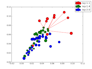
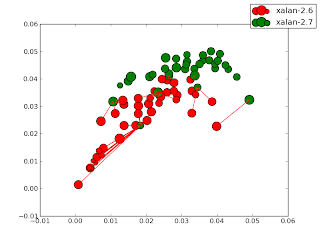
Result1


  • Preliminary feature selection with info gain selecting top 50%
  • Normalized and discredited with Fayyed-Irani
  • PCA via FastMap
  • Grid clustering
  • Centroids plotted along with version n+1 nearest neighbor lines. (Not terribly useful)
  • Do I smell transforms of best fit around the corner?


Results0

k-means 5 to cluster each data-set within itself
Eigenvalues used to determine select features with most influance
Actual selected columns are plotted, not synthesized dimensions
     -- significant correlations could be reported as synonmyms
rules for connecting the dots?


Monday, November 11, 2013

Tree query languages for MOEA

Method

  1. Cluster the data
  2. Find deltas of interest between the clusters
    • Score each cluster
      • Let each row have objective scores, normalized 0..1, min..max
      • Let the score of a row by the sum of the normalized scores
      • Let the score of a cluster be the mean of the score of its rows
      • Technically, this is almost the cdom predicate used in IBEA
    • For each cluster C1
      • Find its nearest neighbor C2 with a better score 
      • Assert one  (leave,goto)  tuple for  (C1,C2)
  3. Build and prune a decision tree on the clusters
    • Label each instance with the cluster it belongs to
    • Build a decision tree on the labelled data set.
    • Find the clusters that are only weakly recognized by the decision tree learner
      • e.g. use a three-way cross val and prune anything with F < 0.5
    • Remove the weakly recognized clusters
  4. For each (C1,C2) tuple where both are not weakly recognized, 
    • Query the tree to find the delta
Observation: the trees are so small that this can be done manually.

Example

Nasa93 clustered into 2D (one color per cluster)

Cluster details 
  • All the following values are normalized 0..1, min..max
  • Defects and months are connected, but not always
  • Effort is not what separates the projects- its more about defects and calender time to develop
  • Clearly, cluster 2 is a bad place and 10 and 13 look nicest.


A decision tree learned from the data labelled with each cluster (ignoring the objectives) generated:

 acap = h
|   apex = h
|   |   pmat = h
|   |   |   plex = h: _2 (6.0/1.0)
|   |   |   plex = n: _4 (3.0)
|   |   pmat = l
|   |   |   cplx = vh: _3 (2.0)
|   |   |   cplx = h
|   |   |   |   time = vh: _3 (3.0)
|   |   |   |   time = n: _6 (4.0/1.0)
|   |   |   cplx = n: _5 (2.0)
|   |   pmat = n: _6 (4.0/1.0)
|   apex = n
|   |   data = h: _6 (2.0/1.0)
|   |   data = n: _4 (3.0/1.0)
|   |   data = l: _13 (1.0)
|   apex = vh
|   |   pcap = h: _10 (3.0)
|   |   pcap = vh: _7 (2.0/1.0)
acap = n
|   sced = n
|   |   stor = xh: _7 (1.0)
|   |   stor = n
|   |   |   cplx = h
|   |   |   |   pcap = h: _10 (3.0/1.0)
|   |   |   |   pcap = n: _13 (3.0)
|   |   |   cplx = n: _7 (3.0/1.0)
|   |   stor = vh: _11 (3.0)
|   |   stor = h: _11 (2.0)
|   sced = l
|   |   $kloc <= 16.3: _9 (5.0)
|   |   $kloc > 16.3: _8 (6.0)
acap = vh: _12 (7.0/1.0)

A 3-way cross-val yielded following confusion matrix. 
  • The underlined and bold entries are the correctly classified rows.
  • The red entries are errors.
  •  Note the poor performance for recognizing clusters 4,5,6,7,10,13

 a b c d e f g h i j k l   <-- as="" classified="" font="">
 5 0 0 0 0 0 0 0 0 0 0 0 | a = _2
 0 4 1 1 0 0 0 0 0 0 0 0 | b = _3
 1 0 2 0 1 0 0 0 1 0 0 0 | c = _4
 0 1 1 0 3 0 0 0 0 0 0 0 | d = _5
 0 1 2 3 0 0 0 0 1 0 0 1 | e = _6
 0 0 0 0 0 0 0 0 1 2 1 1 | f = _7
 0 0 0 0 0 0 6 0 0 0 0 0 | g = _8
 0 0 0 0 0 0 1 4 0 0 0 0 | h = _9
 0 0 1 0 0 0 0 0 3 0 0 2 | i = _10
 0 0 0 0 0 1 0 0 0 4 0 0 | j = _11
 0 0 0 0 0 1 0 0 0 0 6 0 | k = _12
 0 0 1 0 0 0 0 0 1 1 0 2 | l = _13


The above confusion matrix is mapped into the "f" measures of the following table. 
  • The "goto" column marks the deltas of interest.
  •  Low "f" values are marked in gray. 
  • Any "goto" that comes or goes into gray is marked with gray.

cluster n effort defects months f     goto
2 5 43% 25% 72% 91% 3
3 6 5% 32% 42% 67% 6
4 5 6% 17% 37% 31% 8
5 5 7% 29% 43% 0% 6
6 8 6% 24% 40% 0% 10
7 5 7% 16% 36% 0% 13
8 6 2% 6% 17% 92% 9
9 5 0% 1% 3% 89%
10 6 2% 9% 22% 46% 12
11 5 7% 18% 31% 67% 13
12 7 2% 7% 18% 86%
13 5 7% 15% 26% 36%
total: 68


If we prune the above tree of any branch that leads only to gray classes, we get, as promised above, a very small tree.

acap = h
|   apex = h
|   |   pmat = h
|   |   |   plex = h: _2 (6.0/1.0)
|   |   pmat = l
|   |   |   cplx = vh: _3 (2.0)
|   |   |   cplx = h
|   |   |   |   time = vh: _3 (3.0)
acap = n
|   sced = n
|   |   stor = vh: _11 (3.0)
|   |   stor = h: _11 (2.0)
|   sced = l
|   |   $kloc <= 16.3: _9 (5.0)
|   |   $kloc > 16.3: _8 (6.0)
acap = vh: _12 (7.0/1.0)

Summary

  • The definite statements that clearly make changes in SE data are very succinct.
    • But they might not cover everything.
Question: what would you baseline this against? I.e. how would you certify this as a good/crappy idea?