Tuesday, June 12, 2012
Hypothesis 1: Top 25% words from loops FS will best define aptamers.
ie, Informed FSS better than random
Corollary: Random subsets in general will not do well.
1a: Aptamers are not homogeneous and will therefore have multiple groupings within
Hypothesis 2: Aptamers will fall into clusters. Some, but not all, non-aptamers will be outliers and cause error rate to rise. The highest classification error rate will occur in the earliest rounds.
-----------------------------------------------------------------------------------------------------------------------------------
Paper 1 CREATE BENCHMARK, establish that the chosen fss and clusters are accurate for aptamers
Find Representative FSS and CLUSTERS for Aptamers
FIND best FSS and clusters for Full Aptamer DB
LABEL data with best clustering for that subset
TEST with classification accuracy of classifiers
RANK the sets on lowest classification error
P2 APPLY REPRESENTATIVE FSS AND CLUSTERS TO ROUNDS DATA
Apply fss's and centroids to rounds data as a way to discriminate between rounds
Use accuracy or number of additional clusters as measurement of non-aptamers
issues/questions
HOW TO EVAL FSS/CLUSTERS?
how many clusters? or best one?
HOW DO THE OUTLYING INSTANCES INTEGRATE WITH EXISTING
CLUSTERS? new cluster? error?
----------------------------------------------------------------------------------------------------------------------------------
KNOW
Aptamer Db does not easily split and tree. Hard to cluster and j48 not good for classifying
NAIVE BAYES EXCELLENT CLASSIFICATION, JRip, on it's heels with 7-20 rules. 80-90s %
nb > jrip > j48 > decision table >> oneR > zeroR
INFERENCE: Aptamer db follows a predictable distribution. Which one??
IMPLICATION: Use a probabilistic clusterer? ?Try to determine distribution and use goodness of fit for rounds???
Clusters of 10ish+ on Rounds data start to identify areas that are pure.
Both are highly represented in one big cluster.
Need better discriminator.
Full Ellington DB will not cluster
MUST FSS
Reversed strings do differ from it's forward counterpart
Association rules are mostly for one cluster, the one that is all zeros.
So, at it's current configuration - crap
?Would the rules generated from the loops db be valuable???
----------------------------------------------------------------------------------------------------------------------------------
HAVE
Constructed multiple smart and random subsets
and have stats on them
Don't have rig completed to test all fss, clusters, classify
- wanted to explore to make sure this could work before running big experiment
Read Research papers
Word occurance
Using association rules for clustering
DB: Full Ellington DNA Aptamer
Loop DB subset
Two sets of Rounds data with 4-6 rounds of 30 ish instances

Monday, June 11, 2012
Active Learning on Defect Paper
I ran all the data sets through weka's Bayes and Random Forest learners. The g-values produced by weka are very close to the g-values given by my implementation, but I still kept the g-values of weka. The figures are placed together in an under-construction version of the paper.
Monday, May 21, 2012
Rapid recursive spectral learning (RRSL):
Executive summary:
- For our current rig, we have a new optimizer that does interesting things for 2-d goals.
- If we added more dimensions to the goals, then we'd may some really interesting results.
- Abdel:
- We need those distributions for size, effort, defects, have we done this before. That would blow us out to 6-d.
- We need to baseline this against something else. GAs? DEs?
Rapid recursive spectral learning (RRSL):
- A spectral learner learns important parameters by reflecting over training data’s eigenvectors.
- If applied recursively, this approach generates a tree of clusters where each split is defined in terms of the principle component of the data at that level of the tree .
- Traditional recursive spectral learners are slow since the matrix calculations of PCA take polynomial time. Our rapid RRSL algorithm splits data on parameters found by a very fast Nyström approximation [1].
- Any any level in the recursion, RRSL finds two distant points then divides the data on the median position between them. RRSL checks if one these two points dominates the other. If so, then it prunes the dominated half of the data.
- For each leaf cluster generated after domination pruning, RRSL sorts attribute ranges according to how much more frequently they occur in the leaf cluster (compared to the rest of the data). RRSL then generates contrast rules from the first i-th items in that sort. The rules are then applied to data not used in training.
For example:
Recursive spectral learning
Here's RRSL working of a 2-d objective space from feature maps (the goal is most features with fewest violations). In the following:- the thickest black line is the first found dimension
- each thinner line represents a binary split of some thicker line.

Domination pruning
After applying domination pruning, we only get the following eight classes:
Range sorting
When RRSL took one of the above clusters and sorted attribute ranges (bu how more often it appears in that cluster vs anything else), we get the following (this list is sorted most important at the top to least important at the bottom).(Aside: Curiously most of the advise is about what not to do.)(_ID_192 0)
(REGISTRATION_ENFORCEMENT 1)
(REGISTRATION 1)
(_ID_14 1)
(_ID_13 1)
(CUSTOMER_PREFERENCES 0)
(WISH_LIST_CONTENT 0)
(SHIPPING_OPTIONS 0)
(_ID_92 0)
(_ID_193 0)
(_ID_237 0)
(_ID_89 0)
(_ID_226 0)
(_ID_73 0)
(PERMISSIONS 0)
(_ID_191 0)
(_ID_233 0)
(_ID_194 0)
(_ID_187 0)
(_ID_186 0)
(_ID_190 0)
(_ID_189 0)
(PREVIOUSLY_VISITED_PAGES 0)
(_ID_196 0)
(DISCOUNTS 0)
(_ID_239 0)
(_ID_76 0)
(_ID_90 0)
(_ID_75 0)
(_ID_68 0)
(_ID_77 0)
(TARGETING_CRITERIA_PREVIOUS_PURCHASES 0)
(WISH_LIST 0)
(_ID_53 0)
(_ID_235 0)
(_ID_236 0)
(_ID_88 0)
(_ID_91 0)
(_ID_66 0)
(EMAIL_WISH_LIST 0)
(_ID_69 0)
Contrast set rule testing
If we build rules using the first "x" items in the above list, then generate 10,000 more projects (rejecting any that contradict the rules), we get the following effects.
Note that
- After the first 16 items shown above, further changes become mostly noise.
- In terms of max features with least violations, 6 changes look most interesting.
References
[1] John C. Platt, FastMap, MetricMap, and Landmark MDS are all Nyström Algorithms, Proceedings 10th In. Workshop on Artificial Intelligence and Statistics, 2005..
Tuesday, May 15, 2012
Forbes on DM
A plethora of articles on DM from Forbes.
http://www.forbes.com/special-report/data-driven.html
http://www.forbes.com/special-report/data-driven.html
Tuesday, April 24, 2012
What does zero test tell us about the SEE world?
Here is a detailed report using the Blom correction.
Monday, April 23, 2012
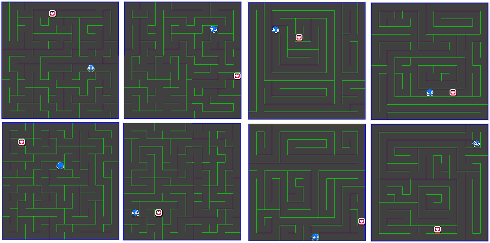
Some PCG Algorithms for Dungeon Generation
Recursive Backtracker Maze Algorithm:
- Go in random unvisited direction and backtrack when each direction is visited until everything is visited
Jar Demo:
http://dl.dropbox.com/u/30075723/joe/RecursiveBacktracker.jar
Jamis Buck Maze Algorithm:
- Similar to Recursive Backtracker
- Addition of some parameters that control bias of turning
Jar Demo:
http://dl.dropbox.com/u/30075723/joe/JamisBuck.jar
Recursive Backtracker (left) versus Jamis Buck (right)
http://www.grabilla.com/02418-29fad28b-4a20-45c7-ab57-6da5bd11f1e5.png
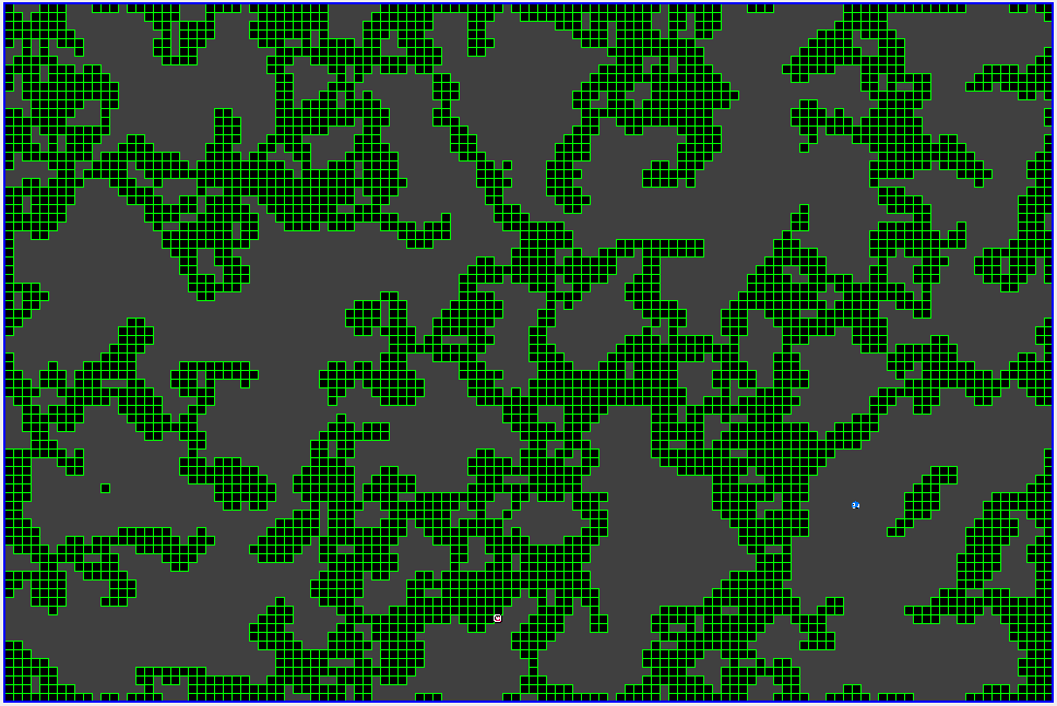
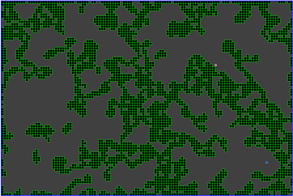
Cellular Automata:
- Change the state of a grid cell (whether it can be walked on or not) based on neighboring states
- If (parameter_above = 5) or more of neighbors are "walkable" then this cell is walkable.
- If (parameter_under = 2) or less of neighbors are NOT "walkable" this this cell is non-walkable.
- Run the above to "erode" the dungeon
- No guarantee of connectedness without further work
Examples of Cellular Automata:
http://www.grabilla.com/02418-3a42a206-b903-439f-986a-55f0b6cb5794.png
http://www.grabilla.com/02418-bfaf95c7-f212-4d47-b5ca-e78217c8a7d8.png
Jar Demo:
http://dl.dropbox.com/u/30075723/joe/CellularAutomata.jar
BSP Tree (Binary Space Partion):
- Split the component in half either vertically or horizontally at some position
- Recurse into each half and repeat until the components are "small enough"
- Add rooms to each resulting component after tree is generated
- Connect rooms (by connecting each component to its sibling)
- Connectedness *is* guaranteed as a property of the BSP Tree
Examples of BSP Tree Dungeons:
http://www.grabilla.com/02418-eab66c9e-2e3b-402a-89df-fcb6ff589c6c.png
http://www.grabilla.com/02418-f73cd867-ae67-4f96-8ad9-861cfee997d6.png
Jar Demo:
http://dl.dropbox.com/u/30075723/joe/BSPTree.jar
- Go in random unvisited direction and backtrack when each direction is visited until everything is visited
Jar Demo:
http://dl.dropbox.com/u/30075723/joe/RecursiveBacktracker.jar
Jamis Buck Maze Algorithm:
- Similar to Recursive Backtracker
- Addition of some parameters that control bias of turning
Jar Demo:
http://dl.dropbox.com/u/30075723/joe/JamisBuck.jar
Recursive Backtracker (left) versus Jamis Buck (right)
http://www.grabilla.com/02418-29fad28b-4a20-45c7-ab57-6da5bd11f1e5.png
Cellular Automata:
- Change the state of a grid cell (whether it can be walked on or not) based on neighboring states
- If (parameter_above = 5) or more of neighbors are "walkable" then this cell is walkable.
- If (parameter_under = 2) or less of neighbors are NOT "walkable" this this cell is non-walkable.
- Run the above to "erode" the dungeon
- No guarantee of connectedness without further work
Examples of Cellular Automata:
http://www.grabilla.com/02418-3a42a206-b903-439f-986a-55f0b6cb5794.png
http://www.grabilla.com/02418-bfaf95c7-f212-4d47-b5ca-e78217c8a7d8.png
Jar Demo:
http://dl.dropbox.com/u/30075723/joe/CellularAutomata.jar
BSP Tree (Binary Space Partion):
- Split the component in half either vertically or horizontally at some position
- Recurse into each half and repeat until the components are "small enough"
- Add rooms to each resulting component after tree is generated
- Connect rooms (by connecting each component to its sibling)
- Connectedness *is* guaranteed as a property of the BSP Tree
Examples of BSP Tree Dungeons:
http://www.grabilla.com/02418-eab66c9e-2e3b-402a-89df-fcb6ff589c6c.png
http://www.grabilla.com/02418-f73cd867-ae67-4f96-8ad9-861cfee997d6.png
Jar Demo:
http://dl.dropbox.com/u/30075723/joe/BSPTree.jar
Tuesday, April 17, 2012
Current Status of Papers
In the Pipeline
- Active learning paper
- Bias variance paper
- LOC comparison paper
- Theoretical Maximum Prediction Accuracy paper
- Active learning for defect
- Tukutuku paper

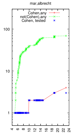
Tuesday, March 20, 2012
LOC-compensation Paper
The latest version of the paper is here. There is still a lot of polishing to do, but the general frame of the paper tells our story (particularly the abstract).
Monday, March 19, 2012
IDEA PROMISE12
ABSTRACT
Background: Most software effort estimation research focuses on methods that produce the most accurate models but very little focuses on methods of mapping those models to business needs.
Aim: Rather than focusing only on algorithm mining, placing the main spotlight on the learner, here we focus on techniques to apply the model in the real world as well. We propose an algorithm called IDEA which creates a dendrogram that can be used to base project parameters decisions to optimize results.
Method: IDEA is compared to 90 solo-methods on 20 datasets using median MRE values. We also show worked examples of how to apply IDEA’s results to project parameter decisions.
Results: By applying IDEA to software effort estimation datasets we generate dendrograms used to make project parameter choices. IDEA does better than most methods 15% of the time, it does just as good as any other method 30% of the time, 35% of the time it does as good as half and 20% of the time it’s in the middle.
Conclusion: IDEA is a linear-time algorithm which can be used effectively to facilitate project decisions and is comparable or better than at least 90 solo-methods tested on 20 effort datasets found in the literature.
Game Surveys
Survey for "League of Legends" now open.
- 69 Results so far, still early in the week.
Survey is here:
http://www.esurveyspro.com/Survey.aspx?id=5cd0fddb-2e5c-451f-bd1e-4dd49e571a1d
Tuesday, March 13, 2012

Idea updates
Modified code to include all Datasets for median plot
http://unbox.org/stuff/var/ray/Plotting/Quartiles/medians.pdfIQR charts for 6 datasets
Dendrograms for all datasets, questions
Monday, March 12, 2012
Grammatech Report
Saturday, March 10, 2012
very fast multiple objective optimization?
This paper
- Ostrouchov, G.; Samatova, N.F.; , "On FastMap and the convex hull of multivariate data: toward fast and robust dimension reduction," Pattern Analysis and Machine Intelligence, IEEE Transactions on , vol.27, no.8, pp.1340-1343, Aug. 2005 doi: 10.1109/TPAMI.2005.164 URL: http://ieeexplore.ieee.org/stamp/stamp.jsp?tp=&arnumber=1453521&isnumber=31215
- Says that "FastMap is a dimension reduction technique that operates on distances between objects. Although only distances are used, implicitly the technique assumes that the objects are points in a p-dimensional Euclidean space. It selects a sequence of k ≤ p orthogonal axes defined by distant pairs of points (called pivots) and computes the projection of the points onto the orthogonal axes. We show that FastMap uses only the outer envelope of a data set. Pivots are taken from the faces, usually vertices, of the convex hull of the datapoints in the original implicit Euclidean space."
That is, the pivots found by Fastmap map out vertexes in the the convex hull (the minimum polygon that contain all points)
Now they don't go the next step (which I think is obvious). To do multi-objective optimization,

- generate candidates
- apply recursive divisive clustering with fastmap, keeping track of all the pviots found along the way
- apply pareto domination to just the pivots, deleting the dominated ones
- use the survivors as parents for the GAs or DEs
- loop
Also, this could be a cache for on-line multi-objective optimization.
- find 1000 examples, recursively cluster them with fastmap.
- Set "important" to be the pivots found in this process
- 1000 times
- find one more example.
- if it falls between pivots, ignore it. else, add it to "important"
- Recursively cluster the important points.
- Set a new "important" set to be the pivots found in this process
- Goto step 2
- Apply the above on-line learner
- When pivots are created, ask an oracle for the value of those pivots.
- And check for domination between each pivot pair
- Only ask the oracle for pivot values
- Watch for new arrivals if they fall outside of a pivot pair
- Only ask the oracle for score on instances that fall outside the pair.
- Check them for domination against the non-dominated 2 pivot pairs
- Forget them if they are dominated
- Else, add them to that "important" set
- Every (say) 1000 instances,
- Forget everything except the non-dominated pivots and the non-dominated newbies.
- Rebuild the cluster tree
Friday, March 9, 2012
This article highlights a possible application for the research I am involved with. Very exciting!
Tuesday, March 6, 2012
Thesis Progress
Chapter 2 (literature review) is currently halfway done at 6 pages + 1. After a quick break to finish deliverables for my classes, I intend to finish the other half by Saturday morning.
The current state of the thesis draft can be found at http://unbox.org/stuff/var/jcraig/thesis/ .
The good news is that the more I read, the more ideas I have as to how things might be done differently. For example, a comparison of NSGA-II against a very similar algorithm, SPEA2, shows that NSGA-II performs better on lower dimensional problems, because it converges a little bit faster than SPEA2. However, SPEA2 does better with higher-dimensional problems, and it gets better distributions. The differences between the two algorithms are so minor that it is a simple matter to tinker with NSGA-II to determine whether it can have SPEA2's distribution while maintaining its speed.
On the local search front, the algorithm EPLS (Evolutionary Parallel Local Search) performs similarly to my modified NSGA-II, but they report performing well against other algorithms (not including NSGA-II, oddly enough). I can try using kNN clustering like they do and using a different breeding operator for the local search like their simplex crossover to see if that gets better results than our clunky FastMap + V-optimal recursive splits with binary uniform crossover.
The current state of the thesis draft can be found at http://unbox.org/stuff/var/jcraig/thesis/ .
The good news is that the more I read, the more ideas I have as to how things might be done differently. For example, a comparison of NSGA-II against a very similar algorithm, SPEA2, shows that NSGA-II performs better on lower dimensional problems, because it converges a little bit faster than SPEA2. However, SPEA2 does better with higher-dimensional problems, and it gets better distributions. The differences between the two algorithms are so minor that it is a simple matter to tinker with NSGA-II to determine whether it can have SPEA2's distribution while maintaining its speed.
On the local search front, the algorithm EPLS (Evolutionary Parallel Local Search) performs similarly to my modified NSGA-II, but they report performing well against other algorithms (not including NSGA-II, oddly enough). I can try using kNN clustering like they do and using a different breeding operator for the local search like their simplex crossover to see if that gets better results than our clunky FastMap + V-optimal recursive splits with binary uniform crossover.
Possibility of Effort Estimates without Software Size
The detailed results are:
- Only instance selection:
- Quick vs. 1NN: 2 losses out of 13 data sets
- Quick vs. CART: 4 losses out of 13 data sets
- Only feature selection:
- Quick vs. 1NN: 4 losses
- Quick vs. CART: 6 losses
- Both feature and instance selection:
- Quick vs. 1NN: 3 losses
- Quick vs. CART: 5 losses
Monday, March 5, 2012
Redesigning Games
The game I made earlier this year: AiMazed
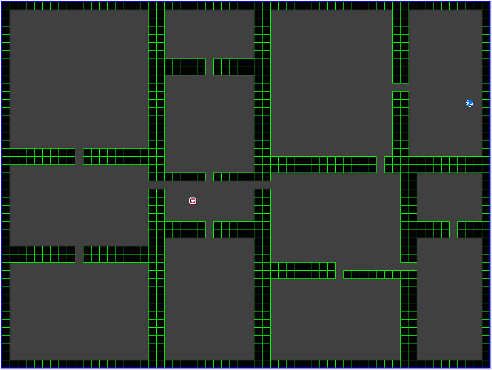
- Random dungeons are built and your job is to pilot a car through the maze and find:
- - - > A key
- - - > An exit
- - - > Enough crystals to power the exit warp
- Meanwhile, there is also an AI computer agent doing the same thing
My (Re)Design Methodology, buffed up a bit:
---Pre-Production of a working version---
- 1. Design the Game
- 2. Guess the AR Vector for your game (AR_PROJECTED) based on your own experience
- - - > 2b. Or, look up an AR Vector from previous knowledge based on the game class/genre
- 3. List each feature in your game
- 4. Score each feature in your game for AR (AR_i)
- 5. Add weights if necessary to the above features
- 6. Average each feature (AR_AVG)
- 7. Compare AR_AVG and AR_PROJECTED
- 8. Add features based on comparison in (7)
--- Post Production of a working version ---
- 9. Discover disruptions to game play and propose fixes to them
- 10. Propose whatever other suggestions you deem appropriate
If the AR_AVG for some aspect is less than that aspect in AR_PROJECTED, then you need to add some features to bring the AR_AVG up to the projection.
Above is put to work to redesign and make AiMazed better.
- This will give us two versions of the game
- Need places (separate places) to post game and get ratings
- Hypothesis: V2 using my method gives a better rating
Tuesday, February 28, 2012
Drafting of the Paper
Not a whole lot yet because of mid-terms last week, plus lost about 2 days when I couldn't get Texmaker installed in Ubuntu properly.
Blarg
Blarg
Idea Supervised vs Unsupervised Win Tie Loss and more
These are Win Tie Loss statistics based on Mann-Whitney for IdeaSupervised and Unsupervised for 20 datasets and below are some initial rankings for Cocomo81s and Kemerer comparing all methods. For the rankings im not sure if they are correct, maybe you could have a look and give me some feedback.

http://dl.dropbox.com/u/7054701/Cocomo81s%20ranking.jpg
http://dl.dropbox.com/u/7054701/Kemerer%20ranking.jpg
Monday, February 27, 2012
Taking Size Out of Data Sets
For the time being I have cocomo, nasa, sdr and desharnais data sets.
The comparison of with-size vs. without-size results for the top13 solo-methods are here.
The comparison of with-size vs. without-size results for the top13 solo-methods are here.
Week in Summary
The 400 Project
> A "master list" of "rules" of game design
Much literature on game design and methodologies. They say to "tune" the game after you design/develop it. But nothing found on methodologies for "tuning".
> Some games involve beta process. Takes in lots of feedback, only one chance to revise.
> Some games have testers who report feedback quickly. Many chances to revise.
> > Testing process draws out and takes time: lots of money.
> Want something that does not involve testers
Working on Qualifier Paper & Presentation
> Section I: History of Gaming and other background information
> > Pre-computing era (Ancient Civilization - 1950)
> > Early Computing Era (1950 - 1980)
> > Computing Era (1980-2000)
> > Golden Age of Gaming (2000 - present)
> Section II: Overview of Games Studies, and Role of Engineering in Games Studies
> Section III: My own research (and what kind of Games Studies it is)
Revise an unsuccessful game into something successful
> Tons of games which are unsuccessful
> Study these games and analyze them
> > What went wrong?
> > Suggest revisions that could have made them successful instead
> I'm currently studying an old game called Deadly Towers
> Coding up a game could take months
> > Working on existing game code involves coding in assembly
Sunday, February 26, 2012
LISP code for differential evolution
For more on
Global Optimisation Algorithms, see
- A general overview;
- Some notes on downhill simplex optimisation.
Wednesday, February 22, 2012
learning for imbalanced data
Learning from Imbalanced Data
Haibo He, Member, IEEE, and Edwardo A. Garcia
Abstract—With the continuous expansion of data availability in many large-scale, complex, and networked systems, such as surveillance, security, Internet, and finance, it becomes critical to advance the fundamental understanding of knowledge discovery and analysis from raw data to support decision-making processes. Although existing knowledge discovery and data engineering techniques have shown great success in many real-world applications, the problem of learning from imbalanced data (the imbalanced learning problem) is a relatively new challenge that has attracted growing attention from both academia and industry.
The imbalanced learning problem is concerned with the performance of learning algorithms in the presence of underrepresented data and severe class distribution skews. Due to the inherent complex characteristics of imbalanced data sets, learning from such data requires new understandings, principles, algorithms, and tools to transform vast amounts of raw data efficiently into information and knowledge representation.
In this paper, we provide a comprehensive review of the development of research in learning from imbalanced data. Our focus is to provide a critical review of the nature of the problem, the state-of-the-art technologies, and the current assessment metrics used to evaluate learning performance under the imbalanced learning scenario.
Furthermore, in order to stimulate future research in this field, we also highlight the major opportunities and challenges, as well as potential important research directions for learning from imbalanced data.
Index Terms—Imbalanced learning, classification, sampling methods, cost-sensitive learning, kernel-based learning, active learning, assessment metrics.
Tuesday, February 21, 2012
Paper Final
Deadline for ICSE-GAS'12 extended to Feb 24.
New Stuff:
- Subdividing Board Gaming data with Rules (Figure 7.)
^ Important when data doesnt match expectations.
Next:
- More Data; Shooter Types and RTS Games
- Another MMORPG and Board Game, to collaborate existing data
- Learn what people think Core and Casual mean (refine data collection)
Monday, February 20, 2012
Saturday, February 18, 2012
Differential Evolution: a Better Optimizer?
Differential Evolution
Differential Evolution: A Survey of the State-of-the-Art Swagatam Das, Ponnuthurai Nagaratnam Suganthan, IEEE TRANSACTIONS ON EVOLUTIONARY COMPUTATION, VOL. 15, NO. 1, FEBRUARY 2011- Compared to most other EAs, DE is much more simple and straightforward to implement. Main body of the algorithm takes four to five lines to code in any programming language. Simplicity to code is important for practitioners from other fields, since they may not be experts in programming and are looking for an algorithm that can be simply implemented and tuned to solve their domain-specific problems. Note that although PSO (particle swarm optimization) is also very easy to code, the performance of DE and its variants is largely better than the PSO variants over a wide variety of problems as has been indicated in many studies.
- As indicated by recent studies, despite its simplicity, DE exhibits much better performance in comparison with several others like G3 with PCX, MA-S2, ALEP, CPSO-H, and so on of current interest on a wide variety of problems including uni-modal, multimodal, separable, non-separable and so on. Although some very strong EAs like the restart CMA-ES was able to beat DE at CEC 2005 competition, on non-separable objective functions, the gross performance of DE in terms of accuracy, convergence speed, and robustness still makes it attractive for applications to various real-world optimization problems, where finding an approximate solution in reasonable amount of computational time is much weighted.
- The number of control parameters in DE is very few (Cr, F, and NP in classical DE). The effects of these parameters on the performance of the algorithm are well- studied. As will be discussed in the next section, simple adaptation rules for F and Cr have been devised to improve the performance of the algorithm to a large ex- tent without imposing any serious computational burden.
- The space complexity of DE is low as compared to some of the most competitive real parameter optimizers like CMA-ES. This feature helps in extending DE for handling large scale and expensive optimization problems. Although CMA-ES remains very competitive over problems up to 100 variables, it is difficult to extend it to higher dimensional problems due to its storage, update, and inversion operations over square matrices with size the same as the number of variables.
Single Objective Differential Evolution
R. Storn and K. V. Price, "Differential evolution: A simple and efficient adaptive scheme for global optimization over continuous spaces," ICSI, USA, Tech. Rep. TR-95-012, 1995. Available: http://icsi.berkeley.edu/~storn/litera.htmlGlobals
- F : combiation factor (try F=0.3)
- Cr : cross over rate (try Cr=0.5)
- NP: number of items in population (try NP=100)
de
function de(NP, F)
   Generate NP random solutions
   for each item P
      value[P] = score(P)
   Stop = false
   while not Stop
     For each item P
        C = candidate(P)
        value[C] = score(C)
        if (better(value[C], value[P]))
           replace P with C
   print BestScore,Best
score
function score(X)
  tmp = objectiveFunction(X)      # domain specific
  if (tmp > Best)
     BestScore = tmp
     Best = X
  if (BestScore >= GoodEnough)
     Stop = true
  Count++
  if (Count > TooMuch)
       Stop = true
  return tmp
candidate
function candidate(original)
  pick three other items at random x,y,z
  candidate = ()
  for each attribute A
     new = x[A]
     if numeric(A)
        new = x[A] + f*([y[A] - z[A]])
     else
        if (rand() < f) new = (rand() < 0.5) ? y[A] : z[A])
     candidate[A] = new
  for each attribute A
     candidate[A] = (rand() < Cr) ? original[A] : candiate[A]
  k = a random attribute
  candidate[A] = original[k] #must use at least 1 parent attribute
  return candidate
Variants
Varitions on a Theme
Storn and Price suggested a total of ten different working strategies for DE and some guidelines in applying these strategies to any given problem.K. Price, R. Storn, and J. Lampinen, "Differential Evolution—A Practical Approach to Global Optimization" Berlin, Germany: Springer, 2005.
_R. Storn and K. Price, "Differential evolution: A simple and efficient heuristic for global optimization over continuous spaces" J. Global Optimization, vol. 11, no. 4, pp. 341-359, 1997. _
None work best in all circumstances. Suck it and see!
Opposition-based DE
When building the candidate, select the opposite value of each numeric range- For an attribute ranging 2..12
- The opposite of 4 is 10
Multiple objective DE
Tea Robic and Bogdan Flipic, 2005.If first standard DE, the candidate is compared to its parent (so the "orginal" is the parent) and there is only a single objective function.
In the next two variant, we allow multiple goals and we apply domination
Domination :  y1 dominates y2 if
    for all objective o, o(y1) <= o(y2)
    and there exists one objective o, o(y1) < o(y2)
- If child dominates, replace original
- If neither doiminates, keep original and add child
The third variant, DEMO/closest/obj, works in the same way as standard, the "original" is the closest item in the objective space.
Tuesday, February 14, 2012
Wilcoxon ranked-sum or Mann-Whitney U test in Bash! on Idea
Idea versus 90 solo methods using the statistical Matt-Whitney U test.

Monday, February 13, 2012
How would data cluster 90 solo-methods
This ad-hoc procedure uses 2 statistical test
The results of the above procedure are incorporated into the jiggle paper on p16-17.
Concise summary of results:
- Wilcoxon Rank Sum Test: To compare 2 arrays of MRE's
- Kruskal-Wallis: To compare n arrays of MRE's
- Sort the solo-methods by their MdMRE's
- Start with j'th group (initially j=1) and place the i'th solo-method into this group
- Compare MRE's of i'th and i+1'th solo-method w.r.t. Wilcoxon
- Compare MRE's of all solo-methods in j'th group and MRE of i+1'th w.r.t. Kruskal-Wallis
- If step3 and step4 both agree that i+1'th method is statistically the same, then place it into j'th group
- Else (if one of step3 or step4 says i+1'th is statistically different), then increment j by 1, i.e. form a new group.
- i = i+1;
- Go to step2
The results of the above procedure are incorporated into the jiggle paper on p16-17.
Concise summary of results:
- Some dataset are awfully flat without any ability to form a second group: telecom and kemerer.
- The datasets that show a good distribution of the solo-methods to their groups is around half the data sets: cocomo81e, nasa93_center_5, desharnais, nasa_93_center_2, sdr, finnish, cocomo81, miyazaki94, nasa93
- The occurrence of the top13 solo-methods within these groups still proves our point, i.e. they are mostly on the top group. However, for certain datasets (desharnaisL3, cocomo81o) the generality does not hold, and the top13 solo-methods occur in lower-performance groups.
- The above result shows that, the generality that we have found from the aggregate of 7 error measures and 20 data sets via win-tie-loss values, still holds when we look at the specifics (just using the MRE's w.r.t. another procedure based on multiple statistical tests). However, we still cannot say that there will be no exceptions due to data sets like desharnaisL3 and cocomo81o.
Aspects of Replayability Paper
Paper Week 4: almost final. Feb 17th submission deadline (Zurich timezone) [ICSE-GAS'12]
New "Game Class diagram":
- Only sensible to compare game-instances with siblings or parents
"JDK Diagrams" = Just Don't Kare (named after Joseph D...err... Henry Krall):
- Used to analyze game data
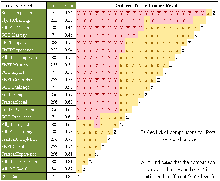
- Offers tukey-kramer analysis, where edges represent statistical indistinguishable-ility
- We only "kare" about nodes which aren't connected, in practice.
Sunday, February 12, 2012
Spectral learning
Spectral learners are those that deal with the eigenvectors of a space.
Why spectra? Well, according to Wikipedia:

So we are doing spectral learning which means that, in theory, our ASE'11 paper could be greatly improved a learner that uses the eigenvectors directly rather than the FASTMAP approximation.
For yet more on spectral learning, see (in stuff/doc):
Note the last paper. The clustering method andrew and me "invented" in 2010 actually dates back to 1998. sigh. our only innovation was to (1) approximate the eigenvectors with fastmap and (2) try it on SE data and (3) compare it to results from the global spalce.
Why spectra? Well, according to Wikipedia:
- A spectrum (plural spectra or spectrums[1]) is a condition that is not limited to a specific set of values but can vary infinitely within a continuum. The word saw its first scientific use within the field of optics to describe the rainbow of colors in visible light when separated using a prism; it has since been applied by analogy to many fields other than optics. Thus, one might talk about the spectrum of political opinion, or the spectrum of activity of a drug, or the autism spectrum. In these uses, values within a spectrum may not be associated with precisely quantifiable numbers or definitions. Such uses imply a broad range of conditions or behaviors grouped together and studied under a single title for ease of discussion.
- In most modern usages of spectrum there is a unifying theme between extremes at either end. Some older usages of the word did not have a unifying theme, but they led to modern ones through a sequence of events set out below. Modern usages in mathematics did evolve from a unifying theme, but this may be difficult to recognize.
- In mathematics, the spectrum of a (finite-dimensional) matrix is the set of its eigenvalues. This notion can be extended to the spectrum of an operator in the infinite-dimensional case.
This idea of the spectrum actually sums up years of my own thinking. SE theory has treated a software project as "one thing" when actually it is a spectrum of things- and we can best study it if we study the data's spectrum).
So, there is a relatively recent newer class of learners that base their reasoning on the eigenvectors. If you don't know what is an eigenvector, they are the invariant properties of a matrix. Its direction, if you will. For example, if we take the eigenvectors of a co-variance matrix, we get the major directions of that data

For more, see http://www.slideshare.net/guest9006ab/eigenvalues-in-a-nutshell or http://www.cs.otago.ac.nz/cosc453/student_tutorials/principal_components.pdf (the first is better for visuals, the second is better for explanatory text).
Now I raise this snince Andrew's learner and the IDEA that Raymond is working with spectra since these are based on Fastmap and...
First published in 1995, FastMap algorithm has been significantly elaborated since then. Wang et al.’s MetricMap algo- rithm tries to replace the iterative projections of Figure 2 with a single multi-profject method [43]. See also the theoretical analysis of Platt that shows that FastMap and MetricMap are really instances of a broader class of what is known as Nystrom algorithms [44]; i.e. they are based on the Nystrom approximation of the eigenvectors of a large matrix.
[43] T. L. Wang, X. Wang, D. Shasha, and K. Zhang, “Metricmap: An embedding technique for processing distance-based queries in metric spaces,” IEEE Transactions on Systems, Man, and Cybernetics, Part B, vol. 35, p. 2005.
[44] J. C. Platt, “Fastmap, metricmap, and landmark mds are all nystro ̈m algorithms,” in In Proceedings of 10th International Workshop on Artificial Intelligence and Statistics, 2005, pp. 261–268.
For yet more on spectral learning, see (in stuff/doc):
- 08spectralLearning.pdf
- 03spectralLearning.pdf
- 05spectralDivisvePartitioning.pdf
- 02_part2_principalDirectionDivisvePartitioning.pdf
- 08farthestCentroidsDivisiveClustering.pdf
- 98principalDirectionDivisvePartitioning.pdf
Note the last paper. The clustering method andrew and me "invented" in 2010 actually dates back to 1998. sigh. our only innovation was to (1) approximate the eigenvectors with fastmap and (2) try it on SE data and (3) compare it to results from the global spalce.


Starting with "why"

Simon Sinek: “people don’t buy what you do, they buy why you do it.”
e.g. Martin Luther King did not say "I have a plan", instead, he said "I have a dream."
e.g. Apple works this way:
e.g. Apple works this way:
- WHY: We exist to think different, to make things better ...
- HOW: ... we are a design company who happens to ...
- WHAT: ... make easy to use computers.
If we find a "why" that other people want, you we can sell our papers, sell our software, sell our careers.
e.g. I have a journal paper with ten times the usual number of citations in that particular journal. That paper had
e.g. I have a journal paper with ten times the usual number of citations in that particular journal. That paper had
- WHY: more people can work together to increase the rigor of our discipline by ...
- HOW: ... using machine learning and a clearer reporting of the results ...
- WHAT: ... using data sets from NASA and algorithms from WEKA, both of which are on-line and you can get running today.
Tuesday, February 7, 2012
This week
We are done with the active learning paper (waiting for reviews). Submission this week.
Read all the available information on Grammatech and placed them here.
Read all the available information on Grammatech and placed them here.
- Question: I have only 3 reports... More stuff to read for me to catch up?
- Question: How to manage the citations? Mendeley is pretty easy to use (see the draft).
Monday, February 6, 2012
Tuesday, January 31, 2012
Idea vs. 90 solo-methods,18 datasets, Ranked by Median MRE

After running Idea.awk through 8 variations of MinSize= 5, 10, 20, 30 and MedianSplit = 0 or 1 and matching it against 90 solo-methods on 18 datasets ranking by Median MRE sorting largest to smallest on each we come up with a median rank of 29.5 for Idea.awk.
| Dataset | Idea MRE Median Rank |
| finnish | 2 |
| telecom1 | 9 |
| kemerer | 12 |
| desharnaisL1 | 13 |
| maxwell | 13 |
| cocomo81o | 17 |
| desharnais | 19 |
| desharnaisL2 | 23 |
| miyazaki94 | 29 |
| desharnaisL3 | 30 |
| nasa93center5 | 35 |
| albrecht | 36 |
| nasa93 | 36 |
| nasa93center2 | 42 |
| cocomo81e | 45 |
| nasa93center1 | 47 |
| cocomo81 | 54 |
| cocomo81s | 75 |
Research week3 idea
View more presentations from rayborg
Monday, January 30, 2012
Delaunay Tessellation
 I have a k-dimensional Delaunay tessellation algorithm based upon the Bowyer-Watson algorithm. It is prototyped in Python, and terribly slow, but I believe that this can be accelerated by magnitudes by using a ball tree.
The next step to seeing whether I can beat NSGA-II is to solve the problem of iteratively generating new solutions that fall within the bounds represented by an individual's nearest neighbors.
Tuesday, January 24, 2012
Concept Lattice Generation
Using a tool called Lattice Miner (written in Java), I was able to generate the following lattices.
NOTE: This lattice was generated using only PD, PF, and PREC as objectives (meaning 3 dimensions). This generated 25 rules. Using all 6 dimensions I have been using (number of bugs found, lines of code, bugs/loc), I was getting 70 rules, which made the lattice chart very large and unwieldy, and therefore not ideal for the presentation:


Limitations: it doesn't allow labelling of edges, only of points.
This tool doesn't have a summary tool (to average the PDs, PFs, etc) that I have found yet.
No command line interface that I have found yet.
Benefits: File structure makes it very easy to generate lattice grid files on the fly
Very quick
Visually appealing
Worth noting: Lattices higher on the tree (towards the top) tend to have higher PD, higher PF, lower precision
As you move down the tree (towards more complicated rules), you start to see lower PF and lower precision, but also lower PD
Subscribe to:
Posts (Atom)