Performance of 'nb' on Winshield Dataset

With 3 classes

With 5 classes

With 10 classes

With 15 classes

With 20 classes

With 37 classes

today

Effect of various Bandwidth&Kernel Combinations in Neighbor Weighting

What is the effect of weighting your neighbors in kNN? Acc. to 3 datasets (Coc81, Nasa93, Desharnais), the effects are as follows:

• Weighting your neighbors acc. to a kernel function creates significantly different results
• However, in these 3 datasets subject to different kernels (Uniform, Triangular, Epanechnikov, Gaussian) and to inverse rank weighted mean (proposed by Mendes et. al.) with various bandwidths, we could not observe an improvement in accuracies.
• Detailed experimental results under http://unbox.org/wisp/var/ekrem/kernel/

Presentation - Finding Robust Solutions to Requirements Models

Presentation to Tsinghua University - Thursday, March 18, 2010.

Based on: Gay, Gregory and Menzies, Tim and Jalali, Omid and Mundy, Gregory and Gilkerson, Beau and Feather, Martin and Kiper, James. Finding robust solutions in requirements models. Automated Software Engineering, 17(1): 87-116, 2010.

Active Machine Learning

Unlabeled data is easy to come by and labeling that data can be a tedious task. Imagine that you've been tasked with gathering sound bytes. All you have to do is walk around with a microphone and you've got your data. Once you have the data you have to label each individual sound byte and catalogue it. Obviously, combing and labeling all the data wouldn't be fun -- regardless of the domain.

Active machine learning is a supervised learning technique whose goal is to produce adequately labeled (classified) data with as little human interference as possible. The active learning process takes in a small chunk of data which has already been assigned a classification by a human (oracle) with extensive domain knowledge. The learner then uses that data to create a classifier and applies it to a larger set of unlabeled data. The entire learning process aims at keeping human annotation to a minimum -- only referring to the oracle when the cost of querying the data is high.

Active learning typically allows for monitoring of the learning process and offers the human expert the ability to halt learning. If the classification error grows beyond a heuristic the oracle can pull the plug on the learner and attempt to rectify the problem...

For a less high level view of Active Machine Learning see the following literature survey on the topic.

Does learning on duplicated or unique defects improve software defect prediction in the nasa mdp data?

The short answer is "no".

Brittleness vs. Number of Classes

The following graph shows the brittleness level of the windshield data set as the number of classes are increased with k-means clustering.

Is kernel effect statistical?

See file kernelWinTieLossValues.xls from http://unbox.org/wisp/var/ekrem/kernel/

In summary:

• Different kernels did not yield a significant difference in performance when compared to each other
• Kernel weighting did not significantly improve the performance of different k values, i.e. there is not a significant difference between k=x and k=x plus kernel

Fastmap: Mapping objects into a k-dimensional space

The Fastmap algorithm turns data-set instances into a k-dimensional coordinate which can be primarily used for visualization and clustering purposes. Given a set of n instances from a dataset, Fastmap operates by doing the following. Assume we're using euclidean distance as the dissimilarity function and that we're operating in a 2-D space.

1. Arbitrarily choose an instance from the set and then find the farthest instance from it. These instances will serve as pivots to map the rest of our instances. Call these objects Oa and Ob. Each incoming instance Oi will be mapped using the line that exists between Oa and Ob.

2. As each new instance enters the space, apply geometric rules to extrapolate the coordinates of the new point.

Using the Cosine Law we can find Xi and then use the Pythagorean theorem to determine the coordinates of Oi as it relates to the line formed between Oa and Ob.

3. From there we can easily turn our coordinates into a visualization or use the coordinates to aid in clustering.

To move from a 2-D space to a k-D space, see http://portal.acm.org/citation.cfm?id=223812

Working With Windshield Data

1. Clustered to determine classes.
2. Found mean pd/pf

http://unbox.org/wisp/var/fayola/forensics/Class_1.pdf

Locality in Defect Prediction

Here, we show how a group of learners performs on 7 of the NASA datasets for software defect prediction both for Within Company and Cross Company.

We also are looking at varying the K for LWL. The greatest change between PD/PF with K values of {5,10,25,50} is 5%, usually around 3%. With changes in PD/PF this small, the actual value of K does not seem to matter.

Two algorithms, Clump and Naive Bayes, are shown both with and without relevancy filtering via the Burak Filter. Although applying the Burak Filter can reduce the variance of the results (for within and cross company when the data is logged), it does not significantly affect the median PD/PF's.

Observing the interaction between PD and PF for all algorithms explored, I cannot see a case where locality is beneficial. The PD vs PF ratio of both the locality based methods and the global methods are almost identical, showing that any gain in PD/loss in PF is at the cost of additional PF/less PD.

Review article on anomaly detection

Varun Chandola, Arindam Banerjee, and Vipin Kumar, "Anomaly Detection : A Survey", ACM Computing Surveys, Vol. 41(3), Article 15, July 2009. 

http://www-users.cs.umn.edu/~kumar/papers/anomaly-survey.php 

IEEE TSE accepts "Genetic Algorithms for Randomized Unit Testing"

Jamie Andrews and Tim Menzies

Randomized testing is an effective method for testing software units. Thoroughness of randomized unit testing varies widely according to the settings of certain parameters, such as the relative frequencies with which methods are called. In this paper, we describe Nighthawk, a system which uses a genetic algorithm (GA) to find parameters for randomized unit testing that optimize test coverage.

Designing GAs is somewhat of a black art. We therefore use a feature subset selection (FSS) tool to assess the size and content of the representations within the GA. Using that tool, we can reduce the size of the representation substantially, while still achieving most of the coverage found using the full representation. Our reduced GA achieves almost the same results as the full system, but in only 10% of the time. These results suggest that FSS could significantly optimize meta heuristic search-based software engineering tools.

Download: http://menzies.us/pdf/10nighthawk.pdf

Webcast: "Finding Local Lessons in SE"

Speaker: Tim Menzies

http://coursecast02.cs.wayne.edu:8080/ess/echo/presentation/d1db6a70-7295-4b90-b1b8-36096cc1d21f

Yet more better ways to do k-means

• Optimize k-means with the triangle inequality
• Alternatives to k-means

Does Kernel Choice Affect Prediction Performance?

What we do with the kernel estimation is to come up with a probability distribution function that is derived from our train data and then use this pdf to assign weights to our neighbors in a kNN approach.

Well when the bandwidths are assigned in accordance with Scott's Rule, we see that at critical regions (where the performance of different methods diverge) kernel weighted selection methods perform better than non-weighted versions. However, for the rest of the graphs, the performance of methods are very close to each other and it is difficult to draw a solid conclusion. Below are the graphs for Desharnais dataset for Triangular, Epanechnikov and Gaussian Kernels respectively.

Classification comparisons using DENSITY

DENSITY is a new classifier I wrote that works by

1. Pruning irrelevant data
2. Set density values using geometric series
3. Rank based on "fairness" class distribution weight

UCI data results: http://unbox.org/wisp/var/adam/results/density/times-accs-pdpf-results.pdf

Defect data results: http://unbox.org/wisp/var/adam/results/density/accuracies

Component vs. Whole Defect Prediction

1. Components trimmed based on number of defective modules (using medians)
2. For each learner..
3. 10X10-way cross val using training sets composed of multiple components vs. varying components

for page, see http://unbox.org/wisp/var/adam/results/defect_dist/datas/mwq

Generality and ``W''

To recap, we've demonstrated that ``W'' is capable of sizable median effort and "spread" reductions in software estimation. I've spent more time getting to know what types of datasets and projects ``W'' is proficient at predicting. Here's some new data:

Two new points to make: I played around with the Desharnais dataset and realized the original synthetic projects where making constraints that represented too few historical projects. The new synthetic project simply makes all independent attributes controllable, and gives results in-line with the other synthetic and non-synthetic project.

Second, multiple-goal NASA93 projects are included. The BFC-NASA93 projects seek to minimize the defects, effort, and months as a whole. The reductions are in-line with the effort-only version of this dataset.

Finally, the big generality statement. To make this somewhat easier to read, I've left it in list format with the frequency counts of each attribute value trailing. I'm still working on a more concise way to express this data, one giant table doesn't seem to help.

key: DATASET.project:::attribute=freq count

NASA93.flight:::acap=25

NASA93.flight:::aexp=6

NASA93.flight:::cplx=13

NASA93.flight:::data=14

NASA93.flight:::lexp=8

NASA93.flight:::pcap=9

NASA93.flight:::rely=20

NASA93.flight:::stor=17

NASA93.flight:::turn=6

NASA93.ground:::acap=16

NASA93.ground:::aexp=9

NASA93.ground:::cplx=13

NASA93.ground:::data=20

NASA93.ground:::lexp=7

NASA93.ground:::pcap=7

NASA93.ground:::rely=18

NASA93.ground:::stor=13

NASA93.ground:::time=14

NASA93.osp2:::sced=87

NASA93.osp:::acap=29

NASA93.osp:::aexp=8

NASA93.osp:::cplx=10

NASA93.osp:::sced=12

NASA93.osp:::stor=24

NASA93.osp:::tool=20

BFC-NASA93.flight:::acap=28

BFC-NASA93.flight:::aexp=2

BFC-NASA93.flight:::cplx=7

BFC-NASA93.flight:::data=15

BFC-NASA93.flight:::lexp=2

BFC-NASA93.flight:::pcap=10

BFC-NASA93.flight:::rely=11

BFC-NASA93.flight:::stor=17

BFC-NASA93.flight:::turn=9

BFC-NASA93.ground:::acap=22

BFC-NASA93.ground:::apex=9

BFC-NASA93.ground:::cplx=4

BFC-NASA93.ground:::data=14

BFC-NASA93.ground:::ltex=10

BFC-NASA93.ground:::pcap=8

BFC-NASA93.ground:::rely=10

BFC-NASA93.ground:::stor=14

BFC-NASA93.ground:::time=11

BFC-NASA93.osp2:::sced=109

BFC-NASA93.osp:::acap=43

BFC-NASA93.osp:::aexp=2

BFC-NASA93.osp:::cplx=17

BFC-NASA93.osp:::sced=13

BFC-NASA93.osp:::stor=16

BFC-NASA93.osp:::team=4

BFC-NASA93.osp:::tool=10

ISBSG-clientserver-discretized.proj1:::Norm_PDF_UFP=9

ISBSG-clientserver-discretized.proj1:::Norm_PDR_AFP=11

ISBSG-clientserver-discretized.proj1:::Projected_PDR_UFP=3

ISBSG-clientserver-discretized.proj1:::Reported_PDR_AFP=4

ISBSG-clientserver-discretized.proj1:::Size_Added=5

ISBSG-clientserver-discretized.proj1:::Size_Enquiry=2

ISBSG-clientserver-discretized.proj1:::Size_File=19

ISBSG-clientserver-discretized.proj1:::Size_Input=16

ISBSG-clientserver-discretized.proj1:::Size_Interface=6

ISBSG-clientserver-discretized.proj1:::Size_Output=4

ISBSG-standalone-discretized.proj1:::Adj_FP=1

ISBSG-standalone-discretized.proj1:::Norm_PDF_UFP=14

ISBSG-standalone-discretized.proj1:::Norm_PDR_AFP=15

ISBSG-standalone-discretized.proj1:::Projected_PDR_UFP=4

ISBSG-standalone-discretized.proj1:::Reported_PDR_AFP=5

ISBSG-standalone-discretized.proj1:::Size_Added=5

ISBSG-standalone-discretized.proj1:::Size_Enquiry=1

ISBSG-standalone-discretized.proj1:::Size_File=13

ISBSG-standalone-discretized.proj1:::Size_Input=17

ISBSG-standalone-discretized.proj1:::Size_Interface=4

ISBSG-standalone-discretized.proj1:::Size_Output=4

ISBSG-standalone-discretized.proj2:::Adj_FP=1

ISBSG-standalone-discretized.proj2:::Norm_PDF_UFP=6

ISBSG-standalone-discretized.proj2:::Norm_PDR_AFP=3

ISBSG-standalone-discretized.proj2:::Projected_PDR_UFP=2

ISBSG-standalone-discretized.proj2:::Reported_PDR_AFP=1

ISBSG-standalone-discretized.proj2:::Size_Input=4

ISBSG-standalone-discretized.proj2:::VAF=2

ISBSG-standalone-discretized.proj2:::Work_Effort=33

MAXWELL.proj1:::T01=9

MAXWELL.proj1:::T02=11

MAXWELL.proj1:::T03=8

MAXWELL.proj1:::T04=4

MAXWELL.proj1:::T05=7

MAXWELL.proj1:::T06=3

MAXWELL.proj1:::T07=23

MAXWELL.proj1:::T08=5

MAXWELL.proj1:::T09=4

MAXWELL.proj1:::T10=7

MAXWELL.proj1:::T11=6

MAXWELL.proj1:::T12=5

MAXWELL.proj1:::T13=4

MAXWELL.proj1:::T14=5

MAXWELL.proj1:::T15=4

coc81.allLarge:::acap=4

coc81.allLarge:::aexp=6

coc81.allLarge:::cplx=3

coc81.allLarge:::data=14

coc81.allLarge:::lexp=5

coc81.allLarge:::modp=1

coc81.allLarge:::pcap=4

coc81.allLarge:::rely=22

coc81.allLarge:::sced=4

coc81.allLarge:::stor=14

coc81.allLarge:::time=5

coc81.allLarge:::tool=4

coc81.allLarge:::turn=6

coc81.allLarge:::vexp=13

coc81.allLarge:::virt=1

coc81.flight:::acap=6

coc81.flight:::aexp=21

coc81.flight:::cplx=7

coc81.flight:::data=18

coc81.flight:::lexp=4

coc81.flight:::pcap=1

coc81.flight:::rely=7

coc81.flight:::stor=27

coc81.flight:::turn=19

coc81.ground:::acap=8

coc81.ground:::cplx=7

coc81.ground:::data=30

coc81.ground:::ltex=2

coc81.ground:::pcap=3

coc81.ground:::pmat=2

coc81.ground:::rely=8

coc81.ground:::stor=30

coc81.ground:::time=9

coc81.osp2:::sced=58

coc81.osp:::acap=4

coc81.osp:::aexp=6

coc81.osp:::cplx=20

coc81.osp:::sced=7

coc81.osp:::stor=23

coc81.osp:::tool=9

desharnais-discretized.proj1:::Adjustment=4

desharnais-discretized.proj1:::Entities=2

desharnais-discretized.proj1:::Language=11

desharnais-discretized.proj1:::Length=3

desharnais-discretized.proj1:::ManagerExp=2

desharnais-discretized.proj1:::PointsAjust=6

desharnais-discretized.proj1:::PointsNonAdjust=3

desharnais-discretized.proj1:::TeamExp=1

desharnais-discretized.proj1:::Transactions=1

desharnais-discretized.proj1:::YearEnd=1

These numbers are out of what was returned after 100 runs, so the total counts within one project might not match another. The take-home here is we've able to maintain these large effort reductions even with widely different recommendations both within the same project and across different projects with similar metrics. Some projects such as OSP2 are every stable, only recommending SCED. Others show some distribution favoring a particular attribute, some seem to get by recommending a small subset of attributes.

Closer study is needed of the attributes returned. Right now I'm not looking at the recommended values, just what attribute was chosen.

Initial Kernel Estimation Plots

• Kernel-based methods are most popular for non-parametric estimators
• They can discover structural features in data which parametric approaches may not reveal
• Kernel performance is measured by AMISE (asymptotic mean integrated squared error)
• Below graphs were produced via Epanechnikov kernel, since Epanechnikov kernel minimizes AMISE
• For below graphs we compute a probability density estimate of a sample vector and then plot the evaluation of this probability density estimate
• Plots (lines) below correspond to probability density function for k=16 from Cocomo81 and Cocomo81 itself respectively. The stars are the sorted effort values of related datasets.

Postcards from CHINA

Greg reports he can halve the median MRE as follows:

1. take data
2. cluster using k=10 means
3. assign a weight alpha to each cluster
4. learn alpha by random sampling (assessing each sample with LSR), selecting best alphas via bore

Results:

• nasa93: median(MRE) now 0.4, was 0.61.
  
• cocomonasa: median(MRE) now 0.39, was 0.64
  

• Nasa93:
          #key, ties, win, loss, win-loss
   oversampled,    0,   1,    0,        1
      original,    0,   0,    1,       -1
  
  cocomonasa:
          #key, ties, win, loss, win-loss
   oversampled,    0,   1,    0,        1
      original,    0,   0,    1,       -1
  
  Combined:
                    #key, ties, win, loss, win-loss
  oversampled|nasa93    ,    1,   2,    0,        2
  oversampled|cocomonasa,    1,   2,    0,        2
  original|nasa93       ,    1,   0,    2,       -2
  original|cocomonasa   ,    1,   0,    2,       -2
  

Learning Treatments for Student Retention using TAR3

Using the treatment learner TAR3 (here, Menzies 2001), treatments were learned from features previously selected from enrollment data experiments. Below are the first obtained treatments:

Class = YES
bestClass = 20.00%

 1 worth=1.112139 [FinAidSTUDENT_AG=[5123.000000..724724.000000]] 
 2 worth=1.105999 [FinAidPARENT_MAR=M] [FinAidSTUDENT_WA=[3878.000000..561500.000000]]   
 3 worth=1.102110 [FinAidFATHER_WAG=[43669.000000..999999.000000]] [FinAidFATHER_ED=3.0]   
4 worth=1.097397 [FinAidPARENT_AGI=[67908.000000..999999.000000]]   5 worth=1.092824 [FinAidSTUDENT_WA=[3878.000000..561500.000000]]   
6 worth=1.092252 [FinAidMOTHER_ED=3.0] [FinAidFATHER_ED=3.0]   
7 worth=1.090565 [FinAidFATHER_WAG=[43669.000000..999999.000000]]   8 worth=1.082257 [FinAidFATHER_ED=3.0]   
9 worth=1.080906 [FinAidMOTHER_WAG=[23139.000000..533395.000000]] [FinAidSTUDENT_AG=[5123.000000..724724.000000]]  
10 worth=1.079164 [TotalClasses=[6.000000..10.000000]] [FinAidPARENT_MAR=M]  

Class = YES
bestClass = 10.00%

 1 worth=1.159171    [FinAidPARENT_MAR=M] [FinAidPARENT_AGI=[67908.000000..999999.000000]] [CUR_ERLHRS=[15.000000..22.000000]] [FinAidSTUDENT_AG=[5123.000000..724724.000000]] 
 2 worth=1.156786    [FinAidFATHER_WAG=[43669.000000..999999.000000]] [FinAidSTUDENT_AG=[5123.000000..724724.000000]]   
3 worth=1.132347    [FinAidPARENT_HOU=4.0] [FinAidSTUDENT_AG=[5123.000000..724724.000000]]   
4 worth=1.128918    [HS_PERCENT=[60.000000..100.000000]] [FinAidMOTHER_WAG=[23139.000000..533395.000000]] [PercentileRankHSGPA=[49.500000..98.400002]]   
5 worth=1.113224    [FinAidSTUDENT_TA=2.0] [HS_PERCENT=[60.000000..100.000000]]   
6 worth=1.112139    [FinAidSTUDENT_AG=[5123.000000..724724.000000]]   7 worth=1.097397    [FinAidPARENT_AGI=[67908.000000..999999.000000]]   8 worth=1.092824    [FinAidSTUDENT_WA=[3878.000000..561500.000000]]   9 worth=1.090565    [FinAidFATHER_WAG=[43669.000000..999999.000000]]  10 worth=1.089154    [ACT1_MATH=[19.000000..510.000000]] [FinAidSTUDENT_MA=U]  

Class = NO
bestClass = 20.00%

 1 worth=1.073376 [PercentileRankHSGPA=[0.000000..49.500000)]  

Class = YES
bestClass = 10.00%

1 worth=1.090117 [ENG10=Y]  

Whole vs. Partial Learning - NASA MDP Components - Part II - Undersampling Vs. Subsampling Vs. No sampling

Experiment stats:

• discretize
• nb, j48
• 10*10-way
• supersampling/undersampling/no sampling vs component vs all

mwu and quarts here

On Profiling RDR (Clump)...

Following are runtime statistics for Bryan's RDR implementation using the JM1 data set (~11000 lines).


As you can easily see NBAYES is the outlier weighing in at a whopping 18.3 minutes. What this tells us is that we're spending way too much time classifying as we go down the tree. What's more is that the data doesn't necessarily change from node to node but what we use to classify (based on our rules) is the variable factor.

Now it's time for the proposal. Since we're using the same information for each classification, why not cache the frequency counts early on and just merge counts when RDR generates a new rule? Once a system like the aforementioned has been implemented, the runtime for RDR would be minimal.

Discretizing W

In my last post, I discovered that the current problem datasets all suffered from an abundance of attribute values. Given that W acts on exact matching for it's query constraints, this causes a problem where nothing is left in the testing set after applying the first constraint. At least in the case of the ISBSG dataset, discretization makes a big difference:

Median Effort Reductions

Median Spread Reductions

For the Desharnais dataset, problems still remain. Even with discretization we can only generate a constrained query 25% of the time. The reported results use 9 discrete bins, but tinkering with this number has yet to see any gains in effort reduction. This is concerning, but currently all Desharnais projects are highly synthetic. A better look at the data is in order.

Awktimization

If you're doing a lot of heavy text crunching with Awk, you've probably found that it can get quite slow very quickly. It always seems to happen whether you program well or not. Unfortunately for us, Awk isn't a very high efficiency tool. But that's not going to stop us. Not today.

You see, the GNU implementation of Awk, gawk, has a built-in profiler that you can use in order to analyze and optimize your Awk scripts. Its beautiful simplicity will cast light on those sinister bottlenecks destroying your performance. To use it, simply call pgawk from the command line on any machine with the GNU Awk installed. (Alternatively, you can pass the --profile option to gawk.) The runtime will execute your script and write the profiler results to a file by default named awkprof.out. This file contains the execution counts for each statement executed in the left margin.

Optimizing the now elucidated bottlenecks in your program should give you a considerable performance boost. However, if after improving on your runtimes, you still find that your program isn't zippy enough, you can put a little bit more spring in its step by compiling it to ANSI C.

That's right, the open-source Awka project takes plain old Awk code and transforms it into a nitroglycerin-breathing, high-performance rocket car written in C. Nested loops, arrays, and user functions benefit the most from the conversion. The final product will typically see performance gains of around 50%, but depending on the code, you could see 300-400% speed boosts.

So if you find that your Awk text crunching just isn't quite up to par, maybe it's time to consider grinding that puppy through a profiler. And if that still isn't enough, give it the Total Language Makeover with a conversion to C. And if you have a problem that's still taking millennia to compute, well, maybe you should contemplate asking a simpler question. :)

1987 Evett Fiber Model

(defn numerator [y x]
(let [m (nrow x)
fnc1 (fn [t u]
(- (/ (* (Math/exp (- u)) (- t 1) (Math/pow u (- t 2)))
(- t 2))
(* (- (Math/exp (- u))) (Math/pow u (- t 1)))))
fnc2 (fn []
(/ (* (- m 1) (+ m 1)) m))
smean (fn [x]
(div (reduce plus x) m))
Sx (fn [x]
(let [vals (div
(reduce plus
(matrix (map #(pow (minus % (smean x)) 2) x))) m)
comat (matrix [[(first vals) 0] [0 (second vals)]])
icomat (matrix [[(second vals) 0] [0 (first vals)]])]
[comat icomat]))]

(/ (/ (fnc1 (/ m 2) (first y)) (* (Math/PI) (fnc1 (/ (- m 2) 2) (first y))))
(mult (pow (det (mult (fnc2) (first (Sx x)))) 0.5)
(Math/pow (+ 1 (mmult (mmult (mult (minus y (smean x)) (fnc2))
(second (Sx x)))
(trans (minus y (smean x)))))
(/ m 2))))))

(defn denominator [y z lamb]
(let [Normal-zlamb (fn [zi]
(* (/ 1 (Math/sqrt (* 2 (Math/PI) (Math/pow lamb 2))))
(Math/exp (- (/ (mmult (minus y zi) (trans (minus y zi)))
(* 2 (Math/pow lamb 2)))))))
SumZ (/ (apply + (map #(Normal-zlamb %) z)) (count z))]
SumZ))

(defn likelihood [x y z lamb]
(/ (numerator y x) (denominator y z lamb)))

Why ``W'' Can't Make Up Its Mind

For the past few weeks, I've been having trouble generating consistent constrained queries in our CBR rig, ``W''. For half the datasets we'd generate recommendations that wouldn't map back to the test set, preventing further analysis. The following char should shed some light on the problem:

For the longest time the concern was with the size of our datasets, given that we weren't returning historical results. Upon closer inspection, the datasets giving us trouble contain a very large number of attribute values, and currently ``W'' only learns single-value constraints. This explains why when we constrain our query from learned data we return no results.

Solution: discretize the data, or build a better matching system.

A Simple Approach to RDR

Gaines and Compton [1] explain Ripple Down Rules pretty simply by analyzing Compton's Reconstruction of the GARVAN ES-1 diagnostic system. GARVAN ES-1 was one of the world's first medical expert systems to be put into routine use and interpreted medical reports for thyroid hormones measurements in blood samples.

The idea behind RDR is combining a dynamic, incremental rule based hierarchy with human experts. Given data and domain specific knowledge, the knowledge based system can make assumptions about a space. The human interaction involved is to repair broken rules created by the system or to provide further insight to the system itself.



Take a look at the GARVAN RDR tree supplied by Gaines and Compton. The system begins at a root node where the first rule (0.00) diagnoses that there isn't an instance of thyroid disease. Obviously this rule is always true so, in decision tree fashion, we follow the 'if-true' link to the next rule 1.46 which attempts to make a better diagnosis. Based on the pass-fail result of the diagnosis, as governed by the human experts, the knowledge based system attempts to refine it's diagnosis as we travel down the tree. In effect, the KBS limits the comparisons and decisions required in knowledge acquisition and maintenance.

You might be thinking, "Hey buddy! What's the big deal, that's just a decision tree!" And it is, but what we're gaining is the strong context provided by the 'if-true', 'if-false' links which strictly contain the addition of new rules. A new rule can only affect conclusions applied to cases previously falling under at most one rule and in general can only affect cases falling under the rule responsible for the conclusion if the new rule were not present. Any rule considered for addition to the system need only be applied underneath one rule.

The structure of the tree allows the computer to take care of all the dirty work, leaving the human designer the capability to apply his/her knowledge effectively within' the framework.

--
[1] Gaines, Brian R., Compton, Paul. Induction of Ripple Down Rules Applied to Modeling Large Databases. University of New South Whales. 1995.

Simple single pass k-means

Farnstrom, F., Lewis, J., and Elkan, C. 2000. Scalability for clustering algorithms revisited. SIGKDD Explor. Newsl. 2, 1 (Jun. 2000), 51-57.  http://portal.acm.org/citation.cfm?id=360419

Model clusters as gaussians:

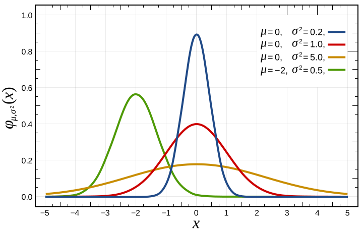
• Clusters are modeled by the  sum, sumSquared, and n of each feature.
• When clusters combine, their new stats are the sum of the of the old sums, the sum of the old symSquareds, and the n 
• Reminder: when x is added to a Gaussian
• n++
• sum = sum + x
• sumSquared = sumSquared + x*x
• mean = sum/n
• sd=  sqrt((sumSquared-((sum*sum)/n))/(n-1)) 
• Do not add a point to a cluster if any of the its attributes falls outside of mean±1.96sd (for 95% confidence) 

Algorithm:

1. Initialize k random clusters C1... Ck
2. Now we have old stats and new stats (initially, old stats is nil)
3. LOOP: Take 1% of the data and add it to a buffer.
4. For all remaining items in the buffer,  run k-means, moving the centroids (until they converge). If can add to a cluster (according to old confidence intervals), then add it (updating sum, sumSquared, and n of new stats).  Here, each cluster is treated as being a point at the mean values, weighted with the number of points in the that cluster.
5. When no more items can be added, then..
1. If any cluster has no items, seed it with the most distant data point
2. Now clear the buffer 
3. Add the new stats to the old stats.
6. If there is no more new data, stop. Otherwise, go to LOOP

Runs nearly twice as fast as old k-means.  Here's the results from using various clustering algorithms on the KDD 1998 cup data (95412 rows, 481 fields). This algorithm is "N1". Normal batch k-means is "K".  "R1" is a random sampling k-means (that, btw, generated low quality clusters).

Note that clusters generated by this algorithms, working in increments of 1% of the data,  produces clusters of almost the same quality as multiple-pass K-means.

Other advantages:

• Small enough memory that you could have multiple versions going, and pick the one with the lowest variances in the generated clusters. 
• Very simple implementation.
• Satisfies the data mining desiderata:

1. Require one scan (or less) of the database if possible: a single data scan is considered costly, early termination if appropriate is highly desirable. 
2. On-line “anytime” behavior: a “best” answer is always available, with status information on progress, expected remaining time, etc. provided 
3. Suspendable, stoppable, resumable; incremental  progress saved to resume a stopped job.
4. Ability to incrementally incorporate additional data with existing models efficiently. 
5. Work within confines of a given limited RAM buffer. 
6. Utilize variety of possible scan modes: sequential,index, and sampling scans if available. 
7. Ability to operate on forward-only cursor over a view of the database. This is necessary since the database view may be a result of an expensive join query, over a potentially distributed data warehouse, with much processing required to construct each row (case).

Searching For Ceiling Effects in NASA MDP Components - Part I - Undersampling

Defect distribution visualization can be found here among components. These are verified by components flagged to be used/ignored based on the median number of defects. Components whose defects exceed in number the median are first filtered for selection. These components can be seen below.

Component ID	Use/Ignore
22295	ignore
22296	ignore
22297	ignore
22298	ignore
22299	ignore
22302	ignore
22303	ignore
22305	ignore
22306	ignore
24952	ignore
24954	ignore
24958	ignore
24959	ignore
24960	ignore
24962	ignore
24964	ignore
24967	ignore
24970	ignore
24971	ignore
25	ignore
25492	ignore
26	ignore
27	ignore
28	ignore
29	ignore
30	ignore
31	ignore
32	ignore
33132	ignore
33135	ignore
33137	ignore
33138	ignore
33139	ignore
33140	ignore
33142	ignore
33143	ignore
33146	ignore
33147	ignore
33148	ignore
34753	ignore
34754	ignore
34755	ignore
34756	ignore
34757	ignore
34758	ignore
34759	ignore
34760	ignore
34761	ignore
34762	ignore
34763	ignore
34764	ignore
34765	ignore
34766	ignore
34767	ignore
34768	ignore
34769	ignore
70812	ignore
70814	ignore
70815	ignore
70818	ignore
70820	ignore
70821	ignore
70822	ignore
70823	ignore
70824	ignore
17	use
18	use
19	use
20	use
21	use
22	use
22292	use
22293	use
22294	use
22300	use
22301	use
22304	use
22307	use
22308	use
22309	use
23	use
24	use
24953	use
24955	use
24956	use
24957	use
24961	use
24963	use
24965	use
24966	use
24968	use
24969	use
25493	use
33133	use
33134	use
33136	use
33141	use
33144	use
33145	use
33149	use
33150	use
34752	use
70816	use
70817	use
70819	use

Plots of the potential ceiling effects can be found here using subsampling, where M=N (#defective = #non-defective). A 10X10-way cross-validation was used in the experiment.

Kernel estimation

Palpanas et al. 2003 Distributed deviation detection in sensor networks (p79)

• Assume a local distribution
• Scream if you do not find it.

But how to assume the local kernel function?

• There are so many.
• Palpanas et al. comment that the actual kernel does not matter. (p79). 
• This is not quite correct. Schneid reports that Wand & Jones reports that the choice of kernel is not as important as choice of bandwidth  (if the sampling bandwidth is high enough, then anything is nearly good enough).

Defect distributions across software components in NASA data

Below are some findings showing the small number of components containing a high density of defects. Note that most components lie below either the red or green lines (average and median respectively), telling us that the majority of components in the data sets shown contain relatively few defects.

KC1 - Ground Control System

PC3 - Flight Software from a current Earth-orbiting satellite

CM1 - Software from a science instrument

Checking prior results in student retention estimation

Prior results in learning predictors for student retention are shown here.

Those reports offer a variety of numbers. But using the Zhang equations, we can computer the missing from the given:

calc(Pos,Neg,Prec,Recall, Pf,Acc) :-
        Pf      is Pos/Neg * (1-Prec)/Prec * Recall, 
        D       is Recall * Pos,
        C       is Pf * Neg,
        A       is C*(1/Pf - 1),
        Acc     is (A+D)/(Neg + Pos). 

Then we can write a simulator to explore a range of possible values. For example, for the Atwell paper:

run(atwel,[prec/Prec,neg=Neg,pos=Pos,pf/Pf,pd/Recall,acc/Acc]) :-
        nl,
        member(Prec,[0.88,0.82,0.73]),
        N   = 5990, 
        Neg = 4881, 
        Pos is (N-Neg), 
        member(Recall,[0.65,0.7,0.75,0.8,0.85,0.9]), 
        calc(Pos,Neg,Prec,Recall,Pf,Acc).

When we run this, we get the following numbers. Note the suspiciously low false alarm rates:

[who=atwel, prec=88, neg=4881, pos=1109, pf=2, pd=65, acc=92]
[who=atwel, prec=88, neg=4881, pos=1109, pf=2, pd=70, acc=93]
[who=atwel, prec=88, neg=4881, pos=1109, pf=2, pd=75, acc=93]
[who=atwel, prec=88, neg=4881, pos=1109, pf=2, pd=80, acc=94]
[who=atwel, prec=88, neg=4881, pos=1109, pf=3, pd=85, acc=95]
[who=atwel, prec=88, neg=4881, pos=1109, pf=3, pd=90, acc=96]
[who=atwel, prec=82, neg=4881, pos=1109, pf=3, pd=65, acc=91]
[who=atwel, prec=82, neg=4881, pos=1109, pf=3, pd=70, acc=92]
[who=atwel, prec=82, neg=4881, pos=1109, pf=4, pd=75, acc=92]
[who=atwel, prec=82, neg=4881, pos=1109, pf=4, pd=80, acc=93]
[who=atwel, prec=82, neg=4881, pos=1109, pf=4, pd=85, acc=94]
[who=atwel, prec=82, neg=4881, pos=1109, pf=4, pd=90, acc=94]
[who=atwel, prec=73, neg=4881, pos=1109, pf=5, pd=65, acc=89]
[who=atwel, prec=73, neg=4881, pos=1109, pf=6, pd=70, acc=90]
[who=atwel, prec=73, neg=4881, pos=1109, pf=6, pd=75, acc=90]
[who=atwel, prec=73, neg=4881, pos=1109, pf=7, pd=80, acc=91]
[who=atwel, prec=73, neg=4881, pos=1109, pf=7, pd=85, acc=91]
[who=atwel, prec=73, neg=4881, pos=1109, pf=8, pd=90, acc=92]

Similarly for the delong results. Here's the query:

run(delong,[prec/Prec,neg=Neg,pos=Pos,pf/Pf,pd/Recall,acc/Acc]) :-
        nl,
        Neg is 500,
        Pos is 500,
        member(Prec,[0.57,0.58,0.59]),
        member(Recall,[0.65,0.7,0.75,0.8,0.85,0.9]), 
        calc(Pos,Neg,Prec,Recall,Pf,Acc).

And here's the results. Note the very high false alarm rates and mediocre accuracies.

[who=delong, prec=57, neg=500, pos=500, pf=49, pd=65, acc=58]
[who=delong, prec=57, neg=500, pos=500, pf=53, pd=70, acc=59]
[who=delong, prec=57, neg=500, pos=500, pf=57, pd=75, acc=59]
[who=delong, prec=57, neg=500, pos=500, pf=60, pd=80, acc=60]
[who=delong, prec=57, neg=500, pos=500, pf=64, pd=85, acc=60]
[who=delong, prec=57, neg=500, pos=500, pf=68, pd=90, acc=61]
[who=delong, prec=58, neg=500, pos=500, pf=47, pd=65, acc=59]
[who=delong, prec=58, neg=500, pos=500, pf=51, pd=70, acc=60]
[who=delong, prec=58, neg=500, pos=500, pf=54, pd=75, acc=60]
[who=delong, prec=58, neg=500, pos=500, pf=58, pd=80, acc=61]
[who=delong, prec=58, neg=500, pos=500, pf=62, pd=85, acc=62]
[who=delong, prec=58, neg=500, pos=500, pf=65, pd=90, acc=62]
[who=delong, prec=59, neg=500, pos=500, pf=45, pd=65, acc=60]
[who=delong, prec=59, neg=500, pos=500, pf=49, pd=70, acc=61]
[who=delong, prec=59, neg=500, pos=500, pf=52, pd=75, acc=61]
[who=delong, prec=59, neg=500, pos=500, pf=56, pd=80, acc=62]
[who=delong, prec=59, neg=500, pos=500, pf=59, pd=85, acc=63]
[who=delong, prec=59, neg=500, pos=500, pf=63, pd=90, acc=64]

ssh keys

This guide will give you everything you need to create and start using an ssh key to bypass password authentication. Before you begin, please understand that ssh keys need to be maintained with a high level of security. If your keys were to become compromised for some reason, whomever inherited your keys could potentially break your pass phrase and gain access to your data.

In a safe location, run the following command to generate your key pair:

ssh-keygen -b 4096 -t rsa

You'll immediately be prompted to choose a file name for the key pair. Most commonly, the string 'identity' is used and I suggest using that. Following that, you'll need to enter a pass phrase twice. The end result of running the above command will leave you with two files: 'identity', and 'identity.pub.' One is private, you should just keep this file on your home machine, laptop, or flash drive and the other is public.

Next, back up your current '~/.ssh' folder and create a new one to house your fresh keys.

mv ~/.ssh ~/.ssh-old
mkdir ~/.ssh
mv identity* ~/.ssh/

Once your keys are in place you can run the following command to 'add' your keys and ensure that everything has gone according to plan. Running this will prompt you for your pass phrase.

ssh-add

Now, we need to set up the public part of your key on any remote hosts you want to access without typing your password. If you have an NFS mount on those hosts (like CSEE) you just need to do this in your home directory. ssh into the server or machine in question and if '~/.ssh' does not exist create it. Once created, go to '~/.ssh' and create the file 'authorized_keys'.

cd ~/.ssh && touch authorized_keys

Finally, copy the contents of your 'identity.pub' file into 'authorized_keys' on the remote host. The next time you authenticate (ensuring that you've used 'ssh-add' in advance) you won't need to enter your password.

Binary/Trinary/etc Trees in LaTeX

For all you LaTeX fans out there, thought you might find this interesting. There is a package out there that lets you represent a decision tree in LaTeX using relatively simple code. You can download it here.

Now for a quick example.
\Tree [.A [.true [.B [.true $+$ ] [.false $-$ ] ] ] [.false [.C [.true [.D [.true $+$ ] [.false $-$ ] ] ] [.false $-$ ] ] ] ]

Turns into the image at the left. The only limitations are that each node can have no more than 5 childeren and the whole tree must be less than 20 levels deep.

MESO

In their paper, "MESO: Supporting Online Decision Making in Autonomic Computing Systems", Kasten and McKinley showcase their novel approach to pattern classification. Called MESO (Multi-Element Self-Organising tree), this pattern classifier is designed to support online, incremental learning and decision making in autonomic systems.

Using supervised data MESO uses a novel approach to cluster data. It also unveils a new tree structure to organise the resulting clusters, which the authors call sensitivity spheres.

To create their sensitivity spheres, Kasten and McKinley improved on the long standing leader follower algorithm which creates small clusters of patterns. Basically, a training pattern within a specified distance is assigned to that cluster, otherwise a new cluster is created.

What is the problem with the algorithm: The distance measure which determines the size of the clusters is fixed throughout the clustering process.

In their paper the authors proposed the use of a growth function to remedy this problem.


distance between the new pattern and the nearest sensitivity sphere

scales the result relative to the difference between the current and

Note: the denominator serves to limit the growth rate based on how far the current is from

Once the data is assigned to these clusters or sensitivity spheres, it is then organised into a novel tree structure. Kasten boasts of a tree structure which rather than focussing on putting individual patterns into large clusters close to the root of the tree, he instead places the focus on his sensitivity spheres. He then builds a MESO tree starting at the root node which is home to all the sensitivity spheres. He further explains:

The root node is then split into subsets of similar spheres which produces child nodes. Each child node is futher split into subsets until each child contains only one sphere.

Results

Using the eight datasets in the table below MESO results shows it superiority in terms of speed and accuracy against other classifiers.

POM2

In 2008, Dr. Menzies authored a paper titled "Using Simulation to Investigate Requirements Prioritization Strategies". This paper showed the effects of project and requirement dynamism on the software development processes. In the Spring of 2008, he tasked his Artificial Intelligence class to expand on this model.

Thus, POM2 was born. One of the main differences between POM and POM2 is that POM focused on small teams and small projects. POM2 built its model around the 5 different branches proposed by Dr. Turner and Dr. Boehm. This varied the project size as well as introducing other factors.

• Personnel - The number skill level of the staff
  
• Dynamism - The amount of project change
• Criticality - The impact of failure after deployment
• Culture - How accepting the staff is of change
• Size - The total number of staff across all teams
  

POM2 implimented all of the branches excluding Personnel. With the information available to us, Personnel was a wash. Better people cost more and produced more. Less talented people cost less and produced less. This lead to a near zero effect.

POM2 was then put through a Monte Carlo simulator while a KEYS search engine isolated the interesting areas in the simulator.

The main discovery is that Agile development methods performed as well as or better than Plan based development methods in all areas, especially excelling in dynamic environments. Further research is needed into the Personell and Criticality branches of POM2 to fully flesh out the model.

POM2 was accepted as a short paper to ASE'09. The full version of the paper can be found here, and the short version can be found here.

Bryan Lemon

Bryan is currently a Computer Science Master's student at West Virginia University. He graduated with his BS in Computer Science from Bluefield State College in spring of 2008.

He, along with a team of other students at Bluefield State College competed in The Intelligent Ground Vehicle competition in the summer of 2008. They took first place in the Autonomous Challenge and 4th overall.

In the Fall of 2009, he, his advisor, and his classmates submitted a paper to ASE'09 detailing a software process development model. It will be featured as a short paper in November's conference. He is currently developing a Decision Tree based clusterer called Ripple Down Rules.

Bryan plans on going on to the PhD program upon completing his Masters degree. Once all is said and done, maybe he will finally have the time to develop a hobby.

PhotoSketch Combines Art, AI, and Voodoo Magic

AI research is a great field and all, but I occasionally look at our colleagues over in computer graphics and marvel at what they are doing. SIGGRAPH Asia is coming up later this year, and while I'm sure that we'll see all sorts of mind-blowing things, Tao Chen et al from Tsinghua University have decided to get the party started right now.

Their development, PhotoSketch, is a cloud-based app (I hear they are all of the rage these days). It takes a quick, labeled sketch from the user and turns it into a beautiful photograph containing all of the requested elements. This video demonstrates the process:

PhotoSketch: Internet Image Montage from tao chen on Vimeo.

Basically, the app lets you enter any rough sketch, label it, and press the big "go" button. Their algorithm will find images in its database that match the given labels and decide on the most appropriate match by looking at the labels and sizes of the other objects in the sketch (hey - there's the data mining connection). It will them seamlessly merge all of these disparate elements into a single image, match them with a background, and adjust the lighting and shadows into something vaguely realistic. The results look awesome. There is still something a little.. off.. about the examples, but they will let the layperson compete with the gods in internet Photoshop contests.

PhotoSketch

Clojure: Lisp's Next Evolution

Clojure is a new, dynamic programming language that is built upon the rock-solid foundation of the Java Virtual Machine, the industry-standard platform that is the foundation for Java, one of the world's most popular and powerful multi-platform languages. But, why write in Clojure if you want to target the JVM instead of Java? Wouldn't it make more sense to write your project in the language for which the virtual machine was designed?

Enter functional programming at its finest; Clojure doesn't just target the JVM. No, it's much more than that -- it's an implementation of Lisp. It's not your standard Common Lisp, however; it's a highly specialized form of the language. It's designed with everything modern functional programmers have in mind: concurrency, immutability, and perhaps most importantly, portability. That's right: all your current Java classes are compatible with Clojure.

Clojure doesn't stop there. The core data structures are immutable and extensible. Code-as-data has been extended to maps and vectors. Practically everything is abstract. Multimethods foster polymorphic programming. It really is an amazing thing.

To see what I mean, you should really have a look for yourself over at Clojure's website. The MIL already has a project that is built upon Clojure, CLIFF, which uses an embedded version of the language to generate forensics models dynamically.

As a functional programmer, writing in Clojure has been a dream come true. Do yourself a favor and hack something up today. :D

ICSM 2009 Presentation - Relevance Feedback

Sadly, I couldn't make it to the International Conference on Software Maintenance this year. Fortunately for us, our fantastic contributor Sonia Haiduc could attend and present our paper. She did a great job, and there is a ton of interest in the follow-up work.

The abstract:
Concept location is a critical activity during software evolution as it produces the location where a change is to start in response to a modification request, such as, a bug report or a new feature request. Lexical based concept location techniques rely on matching the text embedded in the source code to queries formulated by the developers. The efficiency of such techniques is strongly dependent on the ability of the developer to write good queries. We propose an approach to augment information retrieval (IR) based concept location via an explicit relevance feedback (RF) mechanism. RF is a two-part process in which the developer judges existing results returned by a search and the IR system uses this information to perform a new search, returning more relevant information to the user. A set of case studies performed on open source software systems reveals the impact of RF on the IR based concept location.

Want to try some treatment learning?

Have a difficult problem to solve? Do you want to know the exact factors that lead to a diagnosis? You might be able to apply treatment learning to the problem.

First, read this and this. Those two articles should give you the basic background. For a more in-depth discussion, take a look at this draft.

If you're feeling brave, go grab the source code for either TAR3 or TAR4.1. NASA has recently given us the newest versions of both treatment learners. To run these, your computer will require a C compiler and the Matlab runtime environment.

TAR Source Code

Warning: This code does have bugs and isn't particularly well-documented. It works, but don't shout at us if it occasionally crashes.

Text Mining

Recently, Ourmine was used to perform a large text mining experiment on the following large data sets:

Express schemas: AP-203, AP-214
BBC, BBC Sport
Reuters 
The Guardian, (multi-view text data sets)
20 Newsgroup subsets
The main purpose of the experiment was to determine the overall benefits of using slow clustering/dimensionality reduction methods over heuristic means. To conduct the experiment, two dimensionality reduction methods were used - Tf*Idf and PCA - in conjunction with three clustering methods (a naive K-means, GenIc, Canopy clustering).

Tf*Idf, or term frequency * inverse document frequency, is a fast reduction method that reduces the number of attributes in a text data set by filtering out important terms from unimportant ones. The concept here is to identify the terms that appear frequently in a small number of documents, and infrequently across the entire corpus. This allows us to evaluate how "relevant" terms are to that particular document pertaining to a specific concept.

PCA, or Principal Components Analysis, is a reduction method that treats every instance in a dataset as a point in N-dimensional space. PCA looks for new dimensions that better fit these points. In more mathematical terms, it maps possibly correlated variables into a smaller set of uncorrelated variables, which are called principal components. The following image shows an example of how two dimensions can be approximated in a single new dimension feature, as seen by the dashed line.



K-means is a very slow clustering method used (in this experiment) to cluster documents from each corpus.  It's a special case of a class of EM algorithms, works as follows:

Select initial {\em K} centroids at random;
Assign each incoming point to its nearest centroid;  
Adjusts each cluster's centroid to the mean of each cluster;
Repeat steps 2 and 3 until the centroids in all clusters stop moving by a noteworthy amount;
GenIc is a single-pass, stochastic (fast) clustering algorithm. It begins by initially selecting K centroids at random from all instances in the data. At the beginning of each generation, set the centroid weight to one. When new instances arrive, nudge the nearest centroid to that instance and increase the score for that centroid. In this process, centroids become "fatter" and slow down the rate at which they move toward newer examples. When a generation ends, replace the centroids with less than X percent of the max weight with N more random centroids. Repeat for many generations and return the highest scoring centroids.
Canopy clustering is another heuristic clustering method. Developed by Google, canopy clustering reduces the need for comparing all items in the data using an expensive distance measure, by first partitioning the data into overlapping subsets called "canopies". Canopies are first built using a cheap, approximate distance measure. Then, more expensive distance measures are used inside of each canopy to cluster the data. 
Results
In order to determine the benefit of using each clustering method, cluster purity and similarity are used. When a document's class is given to us, we can determine a cluster's purity by finding how "pure" a cluster is based on the existence of classes per cluster. For instance, if a cluster contains a large number of documents containing a large number of classes, the purity of that cluster is relatively low. However, if a cluster contains a large number of documents with very few classes, we can say that the cluster has a high purity.
Cluster similarity tells us how similar documents are either within (intra-cluster similarity) a cluster, or across many clusters (inter-cluster similarity). Thus, we strive for a very high intra-cluster similarity, but a very low inter-cluster similarity based on the concept that clusters are meant to group documents together based on how "similar" they are, therefore we don't want a clustering solution to group documents together that are in no way similar to one another.
The results of this experiment are astounding. The following table represents cluster similarities in relation to runtimes normalized to the more rigorous methods (as these were assumed to perform the best).


Reducer and Clusterer
Time
Intersim
Intrasim
Gain
TF-IDF*K-means
17.52
-0.085
141.73
141.82
TF-IDF*GenIc
3.75
-0.14
141.22
141.36
PCA*K-means
100.0
0.0
100.0
100.0
PCA*Canopy
117.49
0.00
99.87
99.87
PCA*GenIc
11.71
-0.07
99.74
99.81
TF-IDF*Canopy
6.58
5.02
93.42
88.4
 

In this table, "Gain" is the value of the intra-cluster similarity minus the value of the inter-cluster similarity. Thus, a higher gain represents a better overall score for that particular clusterer and reducer. As can be seen, most methods lie below the more rigorous methods (PCA*K-means). However, TF-IDF produces better results than does PCA on most combinations, and by observing TF-IDF*GenIc, we can see that even though is scores second in the table, its runtime is about 1/5-th that of TF-IDF*K-means.
Links to graphs of overall weighted cluster purities are found below for the BBC and BBCSport data sets.  As we can see, in BBCSport, slower methods (K-means) provides the highest cluster purity. However, in BBC we can see that GenIc gives us results that are very close to those of slower solutions. 
BBC purities 
BBC Sport purities