Tuesday, January 24, 2012

Repairing feature models


From http://www.splot-research.org/

INPUT:
   <feature_model name="My feature model">     <-- feature model start tag and name attribute (mandatory)
  <meta>                                                                  <-- Optional
  <data name="description">Model description</data>                 <-- Optional
  <data name="creator">Model's creator</data>                       <-- Optional
  <data name="email">Model creator's email</data>                   <-- Optional
  <data name="date">Model creation date</data>                      <-- Optional
  <data name="department">Model creator's department</data>         <-- Optional
  <data name="organization">Model creator's organization</data>     <-- Optional
  <data name="address">Model creator's address</data>               <-- Optional
  <data name="phone">Model creator's phone</data>                   <-- Optional
  <data name="website">Model creator's website</data>               <-- Optional
  <data name="reference">Model's related publication</data>         <-- Optional
  </meta>
  <feature_tree>                <-- feature tree start tag
    :r root (root_id)                 <-- root feature named 'root' with unique ID 'root_id'         
      :o opt1 (id_opt1)               <-- an optional feature named opt1 with unique id id_opt1
      :o opt2 (id_opt2)               <-- an optional feature named opt2, child of opt1 with unique id id_opt2
      :m man1                         <-- an mandatory feature named man1 with unique id id_man1
        :g [1,*]                      <-- an inclusive-OR feature group with cardinality [1..*] ([1..3] also allowed)
          : a (id_a)                  <-- a grouped feature name a with ID id_a
          : b (id_b)                  <-- a grouped feature name b with ID id_b
            :o opt3 (id_opt3)         <-- an optional feature opt3 child of b with unique id id_opt3
          : c (id_c)                  <-- a grouped feature name c with ID id_c
        :g [1,1]                      <-- an exclusive-OR feature group with cardinality [1..1]
          : d (id_d)                  <-- a grouped feature name d with ID id_d
          : e (id_e)                  <-- a grouped feature name e with ID id_e
            :g [2,3]                      <-- a feature group with cardinality [2..3] children of feature e
              : f (id_f)                  <-- a grouped feature name f with ID id_f
              : g (id_g)                  <-- a grouped feature name g with ID id_g
              : h (id_h)                  <-- a grouped feature name h with ID id_h
  </feature_tree>               <-- feature tree end tag (mandatory)
  <constraints>                 <-- extra constraints start tag (mandatory)
    c1: ~id_a or id_opt2        <-- extra constraint named c1: id_a implies id_opt2 (must be a CNF clause)
    c2: ~id_c or ~id_e          <-- extra constraint named c2: id_c excludes id_e (must be a CNF clause)
  </constraints>                <-- extra constraint end tag (mandatory)
</feature_model>                <-- feature model end tag  (mandatory)


Important:
  • Tags are optional but encouraged
  • Feature tree must have at least one feature, i.e., the root node
  • Extra constraints are optional
  • Each extra constraint must be a CNF clause (any arity)

State of the art in checking these models:
  • A Performance Comparison of Contemporary Algorithmic Approaches for Automated Analysis Operations on Feature Models
    Richard Pohl, Kim Lauenroth and Klaus Pohl. IEEE ASE 2011
 Exponential runtimes


also; just says "no" and maybe offers one counter example


here, a linear-time greedy bayes search (think simpler than W2) generates this in 6 seconds in awk from 10,000 random models from a 300+ class system

Output:
                                                  MEDIAN      N    treatment
                                                  ------    ---    ---------
[                                ------ | ------   ] 80 | 10000    all rows
[                                     ----|  ---   ] 85 |  4945    _id_35 = 1
[                                       ---  |--   ] 90 |  2521    _id_32 = 1
[                                       ---  |--   ] 90 |  2213    _id_68 = 0
[                                       ---  |--   ] 90 |  1903    _id_63 = 0
[                                       ---  |--   ] 90 |  1427    _id_77 = 0
[                                       ---  |--   ] 90 |   711    _id_15 = 1
[                                       ---  | -   ] 90 |   355    _id_17 = 1
[                                       ---  | -   ] 90 |   170    _id_22 = 1
[                                       ---  | -   ] 90 |    86    _id_86 = 0
[                                       ---  |--   ] 90 |    47    _id_24 = 1
[                                       -----| ----] 90 |    20    _id_3 = 0 


What's fun here is that it is telling us what to do and what not to do.
 

CHALK Weekly Progress

Erin's weekly report

Idea's MRE 0, 25, 50, 75 and 100th Percentile Results

Here are Idea's MRE results for 19 datasets since I'm missing sdr, I also added them to Ekrems MRE .CSV file results. But still working on ranking them against Ekrems results. Installed node.js and Node Packet Manager as well as coffeescript. Translated bootstrap.coffee to javascript but still haven't managed to understand it fully. Haven't been able to run bootstrap.coffee either. Looked over wilcoxonTest.awx, mwuTest.awk as well but no success.


Monday, January 23, 2012

Intrinsic Complexity of SEE

How complex should a learner working on SEE data sets be? Our intuition is that there is a need for complex learners, if the data set has enough complexity to it, i.e. if the data set can be divided into complex and self-contained regions. On the other hand, if most of the data is noise and if the data sets can be summarized with only a small number of instances and features, then there is no need for complex learners. The updated version of the QUICK paper investigates this question. The new version with all the results/figures updated is here.

Preview of the Paper ["First" Draft]

Conference: Games and Software Engineering 2012.
Location: Zurich Switzerland. (Part of ICSE 2012.)
Due Date: Feb. 17th

Tuesday, January 17, 2012

What I read this week

CHALK proposal

Li H, Homer N. A survey of sequence alignment algorithms for next-generation sequencing. Brief Bioinform 2010;11:473-483.

- hash tables, spaced seed, q-gram filter, multiple seed hits, suffix/prefix tries, seed extension, suffix trie, FM-index, inexact matches, gapped alignment,

- Aligning sequence reads: gapped alignment, paired-end and mate-pair mapping, base quality, long-read aligner, capillary read aligner, SOLiD reads, bisulfite-treated reads, spliced reads, realignment

- Speed, memory considerations

Revital Eres, Gad M Landau, Laxmi Parida. Permutation pattern discovery in biosequences.Journal of computational biology a journal of computational molecular cell biology 2004 11 (6) p. 1050-1060

- sliding window technique for pattern matching with examples

Smith TF, Waterman MS. Indentification of common molecular subsequences. J Mol Biol 1981;147:195-7.

- Similarity (homology) measure

Smith TF, Waterman MS. Comparison of Biosequences. Advances in Applied Mathematics 1981;489:482-489.

- More detailed algorithm for the Smith-Waterman homology measure, comparison to Sellers and Needleman and Wunsch algorithms

MacIsaac KD, Fraenkel E (2006) Practical strategies for discovering regulatory DNA sequence motifs. PLoS Comput Biol 2(4): e36. DOI: 10.1371/journal.pcbi0020036

- DNA Encoding Schemes with examples

o consensus sequence of preferred nucleotides (ACGT)

o position weight matrix (PWM)

o example: seq to pwm 6 positions

- Clustering of DNA - techniques, dimensionality

o k-medroids

o SOM,

o hierarchical clustering to the motifs and combined clusters with a similarity exceeding 70% by computing a consensus sequence

- Distance / similarity measure for DNA sequences

o fraction of common bits as a similarity metric

o Pearson correlation coefficient between motif PWMs as the similarity measure

Next week:

I need to understand basics of DNA, Computational Chemistry, and Bioinformatics better. I have a few book chapters downloaded from the WVU libraries electronic collection.

Core Games and Casual Games

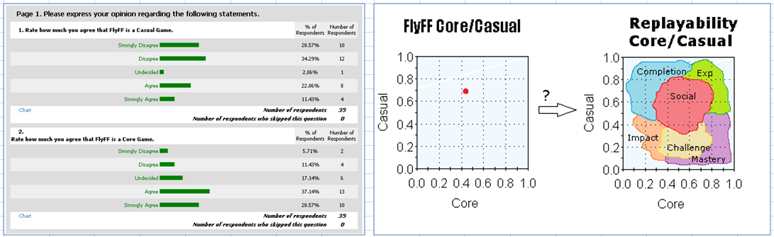
No person is entirely a casual or core gamer, nor can you define them as “50% casual, 50% core.” What about games?

Some people have mixed opinions about the nature of the games they love to play. Survey on FlyFF: http://www.esurveyspro.com/Survey.aspx?id=92c00c57-ee20-4047-9ed4-100fae8b7644


From that, perhaps we can assign replayability-aspect importance to different core-casual scores.

Frustration with concept Lattices

I've been trying to implement this:
http://www.gbspublisher.com/ijtacs/1010.pdf

Unfortunately, I just haven't been able to so far. Hopefully have something by the meeting.

First week of research

Tuesday, January 10, 2012

Virtual Machine and You: A match made in coding heaven

Here's the link to set up Ubuntu Virtual Machine, you crazy coders you:


From here, go to Projects->Homework 1

E-mail me if you have questions.

Monday, January 9, 2012

NSGA-II


Original takes about 900 ms.


Clustered takes about 1100 ms.

Friday, December 16, 2011

Monday, December 5, 2011

unsupervised learning results

nasa93
> ,kloc,0
> ,acap,0.22927988981346761332
> ,data,0.2334438373917348819
> ,time,0.25423355037952316549
> ,plex,0.26866055225810964169
> ,stor,0.27441589382858594393
> ,pmat,0.3093114132807298633
> ,cplx,0.34470954768369121979
> ,apex,0.35198812495229314656
> ,pcap,0.36553252022821636213
> ,rely,0.40329996377433946497
> ,ltex,0.46603801062070232542
> ,pvol,0.56369464132541236001
> ,sced,0.58780717952192207409
> ,tool,0.82277351898917538975
> ,docu,1
> ,flex,1
> ,pcon,1
> ,prec,1
> ,resl,1
> ,ruse,1
> ,site,1
> ,team,1
coc81
> ,tool,0
> ,acap,1
> ,aexp,1
> ,cplx,1
> ,data,1
> ,dev_mode,1
> ,lexp,1
> ,loc,1
> ,modp,1
> ,pcap,1
> ,project_id,1
> ,rely,1
> ,sced,1
> ,stor,1
> ,time,1
> ,turn,1
> ,vexp,1
> ,virt,1
desharnais
>> ,YearEnd,0
>> ,Adjustment,1
>> ,Entities,1
>> ,Langage,1
>> ,Length,1
>> ,ManagerExp,1
>> ,PointsAjust,1
>> ,PointsNonAdjust,1
>> ,Project,1
>> ,TeamExp,1
>> ,Transactions,1
finnish
>> ,prod,0
>> ,at,1
>> ,co,1
>> ,FP,1
>> ,hw,1

nasa93n
>> ,prec,0
>> ,flex,0.11243402160650950439
>> ,docu,0.33052121547798030132
>> ,resl,0.40212091296737206836
>> ,apex,0.46229399349528710328
>> ,data,0.46229399349528710328
>> ,acap,0.61482323785435888386
>> ,pvol,0.61482323785435888386
>> ,sced,0.61482323785435888386
>> ,stor,0.61482323785435888386
>> ,cplx,0.70398054754829086921
>> ,kloc,0.78682242656022605143
>> ,ltex,0.78682242656022605143
>> ,pcap,0.78682242656022605143
>> ,pmat,0.78682242656022605143
>> ,rely,0.78682242656022605143
>> ,ruse,0.78682242656022605143
>> ,team,0.78682242656022605143
>> ,time,0.78682242656022605143
>> ,tool,0.78682242656022605143
>> ,plex,0.87700247550119436735
>> ,site,0.87700247550119436735
>> ,pcon,1

china
>> ,Duration,0
>> ,Resource,0.18076822524622718213
>> ,Enquiry,0.70229300937753547096
>> ,Added,0.70418156239280693676
>> ,NPDR_AFP,0.71748509491228684709
>> ,AFP,0.84023872986505276916
>> ,N_effort,0.84023872986505276916
>> ,Interface,0.85325277904975838084
>> ,File,0.9226111617867434056
>> ,Input,0.94562919153491631352
>> ,Output,0.96948001254205484756
>> ,Changed,0.98391349972332420304
>> ,Deleted,1
>> ,Dev.Type,1
>> ,ID,1
>> ,NPDU_UFP,1
>> ,PDR_AFP,1
>> ,PDR_UFP,1

miyazaki94
>> ,KLOC,0
>> ,FORM,0.40638957366031353002
>> ,ESCRN,0.43471405099857385324
>> ,EFILE,0.63742030743007560556
>> ,FILE,0.74270091796517645477
>> ,EFORM,0.89605538051121036425
>> ,SCRN,1

MRE results

Just listening to the best X percent of attributes, sorted by entropy.
#data sets        cutoff a  ignore           0   25   50    75     100
----------------  ------ -  -------------   ---  ---  ----  ----   ----
data/nasa93.arff, 0.25,  5, 1, , , 10, 0, |, 0,  0.6, 0.81, 0.91,  9.99
data/nasa93.arff, 0.33,  7, 1, , , 10, 0, |, 0, 0.51, 0.77, 0.89,  7.33
data/nasa93.arff,  0.5, 11, 1, , , 10, 0, |, 0, 0.35, 0.69, 0.85, 33.08
data/nasa93.arff, 0.66, 15, 1, , , 10, 0, |, 0, 0.37, 0.61, 0.84,     7
data/nasa93.arff, 0.75, 23, 1, , , 10, 0, |, 0,  0.4, 0.63,  0.9,  12.5
data/nasa93.arff,    1, 23, 1, , , 10, 0, |, 0, 0.42, 0.63, 0.83,  7.33
data/desharnais.arff, 0.001,  1, 1, , , 10, 0, |, 0, 0.34, 0.46, 0.65, 5.92
data/desharnais.arff,  0.25, 11, 1, , , 10, 0, |, 0, 0.22, 0.37, 0.56, 3.87
data/desharnais.arff,  0.33, 11, 1, , , 10, 0, |, 0, 0.25, 0.37, 0.56, 3.87
data/desharnais.arff,   0.5, 11, 1, , , 10, 0, |, 0, 0.25, 0.37, 0.56, 3.87
data/desharnais.arff,  0.66, 11, 1, , , 10, 0, |, 0, 0.25, 0.37, 0.56, 3.87
data/desharnais.arff,  0.75, 10, 1, , , 10, 0, |, 0, 0.27, 0.48, 0.62, 4.18
data/desharnais.arff,     1, 11, 1, , , 10, 0, |, 0, 0.25, 0.37, 0.56, 3.87
 
data/finnish.arff, 0.001, 1, 1, , , 10, 0, |, 0.02, 0.48, 0.71, 0.81, 5.23
data/finnish.arff,  0.25, 1, 1, , , 10, 0, |, 0.05, 0.59, 0.79, 0.85, 4.77
data/finnish.arff,  0.33, 1, 1, , , 10, 0, |, 0.01, 0.58, 0.72, 0.84,  4.9
data/finnish.arff,   0.5, 5, 1, , , 10, 0, |, 0.09, 0.61, 0.76, 0.85,  9.5
data/finnish.arff,  0.66, 5, 1, , , 10, 0, |, 0.09, 0.61, 0.76, 0.85,  9.5
data/finnish.arff,  0.75, 5, 1, , , 10, 0, |, 0.09, 0.61, 0.76, 0.85,  9.5
data/finnish.arff,     1, 5, 1, , , 10, 0, |, 0.09, 0.61, 0.76, 0.85,  9.5
data/coc81.arff, 0.001,   , 1, , , 10, 0, |, 0.07, 0.63, 0.82, 0.98, 15.92
data/coc81.arff,  0.25, 18, 1, , , 10, 0, |, 0.04, 0.76, 0.93,    1, 15.25
data/coc81.arff,  0.33, 18, 1, , , 10, 0, |,    0,  0.6, 0.77, 0.93, 18.58
data/coc81.arff,   0.5, 18, 1, , , 10, 0, |, 0.04, 0.63, 0.86, 0.98,  30.5
data/coc81.arff,  0.66, 18, 1, , , 10, 0, |, 0.04, 0.62, 0.89, 0.99, 27.75
data/coc81.arff,  0.75, 18, 1, , , 10, 0, |,    0, 0.49, 0.85, 0.98, 15.92
data/coc81.arff,     1, 18, 1, , , 10, 0, |,    0, 0.63, 0.84, 0.98, 17.47
data/coc81.arff, 0.001,  1, 1, , , 10, 0, |, 0.04, 0.69,  0.9, 0.98, 14.57
data/coc81.arff,  0.25, 18, 1, , , 10, 0, |,    0, 0.47, 0.82, 0.96, 27.75
data/coc81.arff,  0.33, 18, 1, , , 10, 0, |, 0.01, 0.66, 0.86, 0.98, 15.92
data/coc81.arff,   0.5, 18, 1, , , 10, 0, |, 0.04, 0.58, 0.86, 0.98, 16.96
data/coc81.arff,  0.66, 18, 1, , , 10, 0, |, 0.05, 0.62, 0.94, 1.45, 25.86
data/coc81.arff,  0.75, 18, 1, , , 10, 0, |,    0, 0.62, 0.91, 0.96, 15.92
data/coc81.arff,     1, 18, 1, , , 10, 0, |, 0.06, 0.69, 0.88, 0.99, 15.92
data/miyazaki94.arff, 0.001, 1, 1, , , 10, 0, |,    0, 0.24, 0.45,  0.7,  6.02
data/miyazaki94.arff,  0.25, 1, 1, , , 10, 0, |,    0,  0.2, 0.46, 0.76, 14.25
data/miyazaki94.arff,  0.33, 2, 1, , , 10, 0, |, 0.03, 0.39, 0.61, 0.72, 14.25
data/miyazaki94.arff,   0.5, 3, 1, , , 10, 0, |, 0.01, 0.24, 0.43, 0.63,  4.36
data/miyazaki94.arff,  0.66, 4, 1, , , 10, 0, |,    0,  0.4, 0.61, 0.79,  3.79
data/miyazaki94.arff,  0.75, 5, 1, , , 10, 0, |, 0.02, 0.31, 0.45, 0.72,  3.57
data/miyazaki94.arff,     1, 7, 1, , , 10, 0, |,    0,  0.2, 0.63, 0.78,  5.35
data/china.arff, 0.001,  1, 1, , , 10, 0, |, 0,  0.5, 0.76, 0.94, 93.48
data/china.arff,  0.25,  5, 1, , , 10, 0, |, 0, 0.14, 0.27, 0.45, 14.67
data/china.arff,  0.33,  5, 1, , , 10, 0, |, 0, 0.44, 0.66, 0.83, 46.84
data/china.arff,   0.5,  9, 1, , , 10, 0, |, 0, 0.21, 0.37, 0.58,  8.46
data/china.arff,  0.66, 13, 1, , , 10, 0, |, 0, 0.24, 0.38, 0.59, 13.63
data/china.arff,  0.75, 18, 1, , , 10, 0, |, 0, 0.38, 0.58, 0.76, 12.08
data/china.arff,     1, 18, 1, , , 10, 0, |, 0, 0.37, 0.57, 0.75, 19.35


Comparison of main results from surveys on "all board games together" versus just a single board game: The Settlers of Catan. Social and Impact seem most similar.


Monday, November 28, 2011

Active Learning for Defect Data

Here is a nice report about the active learning experiments.

Monday, November 14, 2011

Replayability Surveys

Survey results for a few types of games:

MMO RPG Game (FlyFF):


Board games:


1. Bias Variance Analysis
    a) Anova -> Bias is 8/20, Variance is 14/20
    b) Scott&Anova -> Bias is 8/20, Variance is 15/20
    c) Anova plus Cohen's correction: Bias is 8/20
    d) Kruskal-Wallis not so good: Bias is 4/20 and variance is 10/20
 
    e) Sorted bias values of all the data sets plotted are here.
           The above plots showed us that there are extreme values due to new experimental conditions.
    f) The Friedman-Nemenyi plots are here for separate data sets.
    g) The same test as before for the entire 20 data sets together are here.
    h) Re-generate boxplots with the new experimental conditions.

I applied a correction on the analysis, because...
Here is the paper with new boxplots..
Here is the Friedman Nimenyi plots on separate data sets, bias is the same for 15 out of 20 data sets..
Below is the result of Friedman Nimenyi over all data sets, i.e. if we see it as 20 repetitions.


2. Papers
    a) HK paper is revised and is ready to be seen here.
    b) Active learning paper's major revision is submitted to TSE.
    c) Camera ready versions of ensemble and kernel papers are submitted to TSE and ESEM.

3. The break-point experiments

Clustering Accelerates NSGA-II


Using a natural clustering method, and replacing poor solutions with solutions bred within "interesting" clusters, appears to accelerate how quickly NSGA-II converges upon the Pareto frontier with little impact on the diversity of the solutions or the speed of the algorithm.

Clusters are divided by heuristically and recursively dividing space along a natural axis for the individuals. The FastMap heuristic is used to pick individuals that are very distant from each other by their independent attributes. All the other individuals are placed in the coordinate space by the magnitude of their orthogonal projections onto the line between the two extreme individuals. A division point is chosen along this axis that minimizes the weighted variance of the individuals' ranks. The splitting continues on each half of the split down to "sqrt(individuals)".

An "interesting" cluster is one that has at least one first-rank individual within it and a low ratio of first-rank individuals to total individuals in the cluster. A "boring" cluster is either completely saturated with first-rank individuals or lower-ranked individuals.

Tuesday, November 1, 2011

Raw data from hall et al

https://bugcatcher.stca.herts.ac.uk/slr2011/

A Systematic Review of Fault Prediction Performance in Software Engineering

http://www.computer.org/portal/web/csdl/abs/trans/ts/5555/01/tts555501toc.htm

http://ieeexplore.ieee.org/xpls/abs_all.jsp?arnumber=6035727&tag=1

stats methids

divide numbers such that the entropy of the treatments they select is minimal: http://unbox.org/stuff/var/timm/11/id/html/entropy.html divide performancescores such that the variance t is minimal: http://unbox.org/stuff/var/timm/11/id/html/variance.html
given N  arrays of performance results p .... of treatments 1,2,3...
with means  m[1],m[2], etc
with stand devs of s[1], s[2], etc then ...

for i in N
   for j in N
        boring[i,j] = (abs(m[i] - m[i])/s <= 0.3) #cohen

samples=1000
N*samples timesRepeat: {
   i = any index 1..N
   j= any index 1..N
  if (boring[i,j] continue
   x = the i-th member of p[i]
   y = the j-th member of p[j]
   diff = x - y
   better = if(errorMeasures) diff<0 else diff>0
   win[i] += better
}
for(i in win)
   win[i] = win[i]/(N*samples) * 100 # so now its percents

rank treatments by their position in win (higher rank = more wins)